39  Integrating single-cell ATAC and RNA

Author

Affiliation

Sean Davis

University of Colorado
Anschutz School of Medicine

A single-cell RNA experiment tells you what each cell is doing: which genes it is actively transcribing, right now, in the moment it was captured. A single-cell ATAC experiment tells you something different and complementary — which stretches of the genome are open for business. ATAC-seq finds the regions of chromatin a cell has unpacked from its tightly wound default state: promoters it has switched on, enhancers it is using, the regulatory switches it has flipped. Expression is the output; accessibility is the wiring that produces it. Measure only one and you are reading half the circuit.

Why does the wiring matter if you can already see the output? Because a cell often opens a regulatory region before, or without, transcribing the gene it controls. A stem cell on the verge of becoming a blood cell can unlock the enhancers of blood-cell genes while those genes are still essentially silent — the chromatin is poised, the decision half-made, but the RNA hasn’t caught up yet. Accessibility therefore carries information about a cell’s trajectory and regulatory state that expression alone misses: which transcription factors are active, which enhancers drive which genes, where a cell is heading rather than only where it is.

The technology that makes this concrete is the multiome assay (here, 10x Genomics’ Single Cell Multiome ATAC + Gene Expression), which measures both RNA and open chromatin in the same nucleus. That “same nucleus” is the crucial part. With separate experiments you can only compare populations — the average RNA of one batch of cells against the average accessibility of another. With a multiome you can ask a cause-and-effect question inside a single cell: this enhancer is open, and this gene, which it controls, is expressed, in this very cell. That is what lets you move from cataloguing cell types to reconstructing the regulatory logic that defines them.

This chapter is about integration: combining the two modalities into one coherent analysis instead of two parallel ones. We will build the intuition for what integration means, why it is harder than it sounds, and then do it hands-on with a public 10x PBMC multiome dataset that ships ready-to-use as a Bioconductor MultiAssayExperiment. For the wider landscape of single-cell multi-omic technologies and the computational methods that pair with them, two reviews are good companions to this chapter (Argelaguet et al. 2021; Vandereyken et al. 2023).

39.1 What you’ll learn

• Why chromatin accessibility (ATAC) and gene expression (RNA) are complementary readouts of the same cell, and what each one uniquely tells you.
• The three shapes of single-cell integration — vertical, diagonal, and mosaic — and how knowing which one you have decides which methods apply.
• The feature-space problem: RNA is measured over genes, ATAC over genomic peaks, and why that mismatch is the central obstacle to integration.
• The bridges that connect the two spaces: gene-activity scores, peak-to-gene links, and transcription-factor motif activity.
• How to load and explore a real multiome dataset as a MultiAssayExperiment of two SingleCellExperiments, and process each modality on its own terms.
• How to build a joint embedding that uses both modalities at once, and what it buys you over either modality alone.

This chapter builds directly on the single-cell RNA-seq chapter (the SingleCellExperiment, normalization, HVGs, PCA/UMAP, clustering) and on the bulk ATAC-seq chapter (peaks, fragments, what accessibility is). If either is hazy, skim it first — we lean on both.

39.2 Two views of the same cell

It helps to be precise about what each assay actually counts.

• scRNA-seq counts transcripts and assigns them to genes. A cell becomes a vector of ~20,000–30,000 gene counts. High counts for a gene mean that gene is being transcribed.
• scATAC-seq counts sequencing fragments that fall in accessible chromatin and assigns them to peaks — genomic intervals (typically a few hundred base pairs) that are open across many cells. A cell becomes a vector of counts over ~100,000+ peaks. A nonzero count for a peak means that region was accessible in that cell.

Two consequences follow immediately, and they drive everything else in the chapter:

1. The two modalities live in different feature spaces. One is indexed by genes, the other by genomic coordinates. You cannot simply stack a gene-by-cell matrix on top of a peak-by-cell matrix and call it integrated — the rows mean different things.
2. ATAC data is sparse and nearly binary. Each cell has at most two copies of any locus, so a peak is essentially “seen” or “not seen” in a given cell. The peak matrix is far sparser than the RNA matrix, which changes how we normalize and reduce it (more on this below — it is why ATAC uses TF-IDF and LSI rather than the log-normalization + PCA you used for RNA).

39.3 What “integration” means: vertical, diagonal, mosaic

“Integrate the ATAC with the RNA” can mean several genuinely different problems, and the single most useful thing you can do before reaching for a tool is to figure out which one you have. The cleanest way to organize them (after Argelaguet et al. (2021)) is by what the two datasets share:

Shape	What’s shared	Typical source	The hard part
Vertical	the same cells, different modalities	10x Multiome (RNA + ATAC per nucleus)	nothing to match — just combine the two views well
Diagonal	different cells, different modalities	a scRNA run and a separate scATAC run	you must infer which cells correspond
Mosaic	partial overlap	some cells multiome, some single-modality	bridge the measured and the missing

The distinction is not academic — it changes the method entirely:

• In vertical integration the correspondence is handed to you. Cell 5’s RNA and cell 5’s ATAC are the same cell, by construction. The task is to learn a single representation that respects both views — a joint embedding. This is the easier, intuition-building case, and where we start.
• In diagonal integration there is no correspondence at all. You have RNA for one set of cells and ATAC for a different set, and nothing tells you that an RNA cell and an ATAC cell are “the same kind.” You must infer the alignment, almost always by projecting both into a shared feature space (the bridges below) and matching. This is the case that forces you to understand why integration is hard, and we return to it in the next chapter using label transfer.

Your collaborators will bring you both. Someone with a 10x Multiome run has a vertical problem. Someone who ran scRNA last year and scATAC this year — same tissue, different cells — has a diagonal one. Same words, “integrate ATAC with RNA,” completely different machinery.

39.4 The feature-space problem and the bridges

Because RNA lives in gene space and ATAC in peak space, every integration method needs a bridge that puts the two modalities into a common frame. There are three bridges worth knowing, and they are not interchangeable — each answers a different question:

• Gene-activity scores. Summarize a gene’s accessibility by summing the ATAC signal over its body and promoter (or, better, distance-weighted nearby peaks). This casts ATAC into gene space, so an ATAC cell can be compared to an RNA cell gene-for-gene. It is crude — accessibility is not expression — but it is the workhorse bridge for aligning unpaired datasets and for annotating ATAC cells from an RNA reference.
• Peak-to-gene links. Correlate a peak’s accessibility against a gene’s expression across cells. A peak whose opening tracks a gene’s expression is a candidate regulatory element for that gene. This is less a bridge for alignment than a biological result — it is how you discover enhancer→gene wiring, and it needs paired (or pseudobulked) data to compute.
• Motif / TF activity. Collapse the tens of thousands of peaks into the handful of transcription factors whose binding motifs they contain (e.g. with chromVAR (Schep et al. 2017)). This turns the unwieldy peak space into a small, interpretable space of TF activities — and TFs are the natural currency for connecting open chromatin back to the genes it regulates.

Keep these three straight and most of the integration literature snaps into focus: methods differ mainly in which bridge they use and whether they need the cells to be paired.

39.5 The data: 10x PBMC multiome

We’ll use a public 10x Genomics dataset of roughly 10,000 peripheral blood mononuclear cells (PBMCs) from a healthy donor, profiled with the Single Cell Multiome assay so that every nucleus has both an RNA and an ATAC measurement. It is a good teaching set: PBMCs contain well-characterized, easily recognized immune cell types (T cells, B cells, monocytes, NK cells), so we have strong priors about what the answer should look like.

Rather than download and reprocess the raw 10x files, we use the curated copy from the Bioconductor SingleCellMultiModal package (Eckenrode et al. 2023), which delivers the dataset as a MultiAssayExperiment — the natural container for “several assays measured on the same cells,” and the multi-modal generalization of the SummarizedExperiment/SingleCellExperiment classes you have already met.

library(SingleCellMultiModal)   # the curated 10x PBMC multiome dataset
library(MultiAssayExperiment)   # the multi-modal container
library(SingleCellExperiment)   # each modality is an SCE
library(Seurat)                 # WNN joint embedding lives here
library(Signac)                 # ATAC processing (TF-IDF / LSI) and ChromatinAssay
library(ggplot2)                # ggtitle() to label the comparison panels
library(patchwork)              # compose plots side by side with `+`

A single call fetches the data (the first time, it downloads from Bioconductor’s ExperimentHub and caches locally; afterwards it loads from the cache):

mae <- scMultiome("pbmc_10x", modes = "*", dry.run = FALSE, format = "MTX")

Working on: pbmc_atac_se.rds

Working on: pbmc_atac.mtx.gz

Working on: pbmc_rna_se.rds

Working on: pbmc_rna.mtx.gz

Working on: pbmc_atac,
 pbmc_rna

see ?SingleCellMultiModal and browseVignettes('SingleCellMultiModal') for documentation

loading from cache

Loading required namespace: HDF5Array

see ?SingleCellMultiModal and browseVignettes('SingleCellMultiModal') for documentation

loading from cache

Working on: pbmc_atac,
 pbmc_rna

see ?SingleCellMultiModal and browseVignettes('SingleCellMultiModal') for documentation

loading from cache

see ?SingleCellMultiModal and browseVignettes('SingleCellMultiModal') for documentation

loading from cache

Working on: pbmc_colData

Working on: pbmc_sampleMap

see ?SingleCellMultiModal and browseVignettes('SingleCellMultiModal') for documentation

loading from cache

see ?SingleCellMultiModal and browseVignettes('SingleCellMultiModal') for documentation

loading from cache

mae

A MultiAssayExperiment object of 2 listed
 experiments with user-defined names and respective classes.
 Containing an ExperimentList class object of length 2:
 [1] atac: SingleCellExperiment with 108344 rows and 10032 columns
 [2] rna: SingleCellExperiment with 36549 rows and 10032 columns
Functionality:
 experiments() - obtain the ExperimentList instance
 colData() - the primary/phenotype DataFrame
 sampleMap() - the sample coordination DataFrame
 `$`, `[`, `[[` - extract colData columns, subset, or experiment
 *Format() - convert into a long or wide DataFrame
 assays() - convert ExperimentList to a SimpleList of matrices
 exportClass() - save data to flat files

The object bundles two experiments measured on the same 10,032 cells:

• rna — a SingleCellExperiment of gene expression counts (~36,500 genes).
• atac — a SingleCellExperiment of peak accessibility counts (~108,000 peaks).

Because they share the same cells, the MultiAssayExperiment keeps their column (cell) metadata aligned for us — this is exactly the bookkeeping that makes vertical integration tractable. We pull out the two modalities to work with each on its own terms:

sce.rna  <- experiments(mae)[["rna"]]
sce.atac <- experiments(mae)[["atac"]]

sce.rna

class: SingleCellExperiment 
dim: 36549 10032 
metadata(0):
assays(1): counts
rownames(36549): MIR1302-2HG FAM138A ... CDY1 TTTY3
rowData names(2): id modality
colnames(10032): AAACAGCCAAGGAATC AAACAGCCAATCCCTT ... TTTGTTGGTTGGTTAG
  TTTGTTGGTTTGCAGA
colData names(6): nCount_RNA nFeature_RNA ... celltype broad_celltype
reducedDimNames(0):
mainExpName: NULL
altExpNames(0):

sce.atac

class: SingleCellExperiment 
dim: 108344 10032 
metadata(0):
assays(1): counts
rownames(108344): chr1:10109-10357 chr1:180730-181630 ...
  chrY:11332988-11334144 chrY:56836663-56837005
rowData names(2): id modality
colnames(10032): AAACAGCCAAGGAATC AAACAGCCAATCCCTT ... TTTGTTGGTTGGTTAG
  TTTGTTGGTTTGCAGA
colData names(6): nCount_RNA nFeature_RNA ... celltype broad_celltype
reducedDimNames(0):
mainExpName: NULL
altExpNames(0):

39.6 From Bioconductor to Seurat: building the joint object

The joint-embedding method we’ll use — weighted nearest neighbors (WNN) — lives in the Seurat/Signac ecosystem (Stuart et al. 2021), which is the de-facto standard for paired multiome. So our first practical step is to bridge our MultiAssayExperiment into a Seurat object: the RNA counts become a standard expression assay, and the ATAC peak counts become a Signac ChromatinAssay. This Bioconductor→Seurat hand-off is worth learning in its own right — you will reach for it constantly, because single-cell data routinely arrives in one ecosystem and the method you want lives in the other.

# RNA becomes a standard expression assay.
pbmc <- CreateSeuratObject(counts = counts(sce.rna), assay = "RNA")

# ATAC becomes a ChromatinAssay, which identifies each peak by its genomic
# coordinates. Peaks can reach us two ways: as a GRanges in the SCE's rowRanges,
# or encoded in the rownames as coordinate strings like "chr1:9776-10668". We
# prefer the GRanges when present and fall back to parsing the rownames.
atac.counts <- counts(sce.atac)
peak.ranges <- tryCatch(rowRanges(sce.atac), error = function(e) NULL)

pbmc[["ATAC"]] <- if (is(peak.ranges, "GRanges") && length(peak.ranges) == nrow(atac.counts)) {
  CreateChromatinAssay(counts = atac.counts, ranges = peak.ranges)
} else {
  CreateChromatinAssay(counts = atac.counts, sep = c(":", "-"))
}
pbmc

An object of class Seurat 
144893 features across 10032 samples within 2 assays 
Active assay: RNA (36549 features, 0 variable features)
 1 layer present: counts
 1 other assay present: ATAC

NoteWe deliberately skip the fragment file

The raw 10x multiome ships a large fragments file (every ATAC fragment, genome-wide). The curated dataset gives us the peak matrix instead, so we build the ChromatinAssay without fragments. WNN needs only the per-modality reductions, so this costs us nothing here — but it does mean genome-browser coverage tracks and fragment-based gene-activity scores aren’t available in this chapter. We don’t need them for the joint embedding.

39.6.1 RNA reduction: the familiar recipe

The expression side is exactly the workflow from the scRNA-seq chapter — normalize, pick highly variable genes, scale, and reduce with PCA:

DefaultAssay(pbmc) <- "RNA"
pbmc <- NormalizeData(pbmc)

Normalizing layer: counts

pbmc <- FindVariableFeatures(pbmc, nfeatures = 3000)

Finding variable features for layer counts

pbmc <- ScaleData(pbmc)

Centering and scaling data matrix

pbmc <- RunPCA(pbmc, reduction.name = "pca")

PC_ 1 
Positive:  SKAP1, BCL11B, CD247, IL32, EEF1A1, CAMK4, TC2N, IL7R, LEF1, BACH2 
       INPP4B, TRAC, LTB, BCL2, ITK, SYNE2, CD96, THEMIS, TRBC2, RORA 
       SLFN12L, TXK, PRKCQ, TNIK, ANK3, STAT4, GRAP2, CCR7, CARD11, TESPA1 
Negative:  PLXDC2, SLC8A1, LRMDA, FCN1, MCTP1, RBM47, TYMP, IRAK3, JAK2, DMXL2 
       NAMPT, TBXAS1, LYN, ZEB2, LRRK2, CYBB, TNFAIP2, SAT1, GAB2, HCK 
       CLEC7A, TLR2, CSF3R, LYST, VCAN, FGD4, GRK3, FAM49A, CD36, MARCH1 
PC_ 2 
Positive:  CD247, BCL11B, IL32, DPYD, TC2N, AOAH, IL7R, TNIK, INPP4B, CAMK4 
       PDE3B, ITK, SLFN12L, TRAC, THEMIS, PRKCQ, RORA, SLCO3A1, LEF1, TXK 
       STAT4, ANXA1, NEAT1, FNDC3B, ARHGAP26, SRGN, CD7, ADGRE5, PLCB1, TRBC1 
Negative:  BANK1, MS4A1, PAX5, NIBAN3, FCRL1, IGHM, AFF3, EBF1, LINC00926, OSBPL10 
       CD79A, RALGPS2, COBLL1, CD22, BLNK, BLK, AP002075.1, IGHD, ADAM28, COL19A1 
       BCL11A, CD79B, PLEKHG1, GNG7, DENND5B, WDFY4, SPIB, AC120193.1, RUBCNL, TCF4 
PC_ 3 
Positive:  MAML2, LEF1, PDE3B, BACH2, CCR7, CAMK4, IL7R, FHIT, NELL2, LTB 
       NR3C2, RASGRF2, INPP4B, MAL, ANK3, IGF1R, MLLT3, CSGALNACT1, TESPA1, PLCL1 
       ITGA6, LINC01550, AC139720.1, BCL2, SLC2A3, PRKN, PATJ, TSHZ2, LEF1-AS1, SESN3 
Negative:  NKG7, GNLY, PRF1, KLRD1, GZMB, GZMA, CST7, CCL5, FGFBP2, SPON2 
       GZMH, ADGRG1, KLRF1, TGFBR3, CCL4, CLIC3, PDGFD, PTGDR, FCRL6, C1orf21 
       IL2RB, PPP2R2B, BNC2, CTSW, TBX21, HOPX, FCGR3A, PYHIN1, CX3CR1, MYBL1 
PC_ 4 
Positive:  PAX5, FCRL1, MS4A1, LINC00926, EBF1, OSBPL10, BANK1, CD79A, CD22, COL19A1 
       CD79B, PLEKHG1, ADAM28, AP002075.1, IGHD, MTSS1, FCER2, MCTP2, IGHM, SWAP70 
       AC120193.1, LARGE1, NKG7, GNLY, RALGPS2, FCRL2, FCRL3, PRF1, KLRD1, STEAP1B 
Negative:  LINC01478, CLEC4C, CUX2, EPHB1, LILRA4, COL26A1, PTPRS, SCN9A, LINC01374, LINC00996 
       AC023590.1, COL24A1, NRP1, PHEX, FAM160A1, TNFRSF21, PACSIN1, SLC35F3, PLXNA4, SCAMP5 
       PLD4, DNASE1L3, LRRC26, PLEKHD1, P3H2, SCN1A-AS1, ITM2C, SCT, PTCRA, SERPINF1 
PC_ 5 
Positive:  CDKN1C, IFITM3, HES4, CSF1R, FCGR3A, SMIM25, MS4A7, LST1, AC104809.2, LRRC25 
       AIF1, AC020651.2, MAFB, CALHM6, CFD, GPBAR1, FMNL2, CTSL, SERPINA1, SIGLEC10 
       TCF7L2, HMOX1, MTSS1, CST3, HLA-DPA1, CKB, TMSB4X, COTL1, SPRED1, CASP5 
Negative:  PLCB1, VCAN, ARHGAP24, CSF3R, DYSF, LINC00937, VCAN-AS1, GLT1D1, ITGAM, FNDC3B 
       PADI4, EIF4G3, PDE4D, AC020916.1, CREB5, TREM1, MEGF9, CD36, ARHGAP26, FCAR 
       VAV3, MICAL2, CLMN, ACSL1, KIF13A, JUN, ANXA1, CRISPLD2, MCTP2, RAB11FIP1 

39.6.2 ATAC reduction: why not PCA, and what TF-IDF + LSI do instead

The accessibility side needs a different reduction, and the reason is the structure of the data. Recall that the peak matrix is sparse and nearly binary: a cell has at most a couple of copies of any locus, so most entries are 0 and the rest are small. Log-normalization-then-PCA, which works well for the graded counts of RNA, is a poor fit for this on/off signal. The fix, worked out for the earliest single-cell ATAC experiments (Cusanovich et al. 2015), borrows two ideas from how search engines compare text documents: TF-IDF, then LSI.

39.6.2.1 TF-IDF, in miniature

TF-IDF stands for term frequency–inverse document frequency. The analogy is to text: if cells are “documents” and peaks are “words,” then a peak open in nearly every cell is like the word the — common, and therefore almost useless for telling documents apart — while a peak open in just a handful of cells is like a rare, distinctive word that pins down which documents resemble each other. TF-IDF rewrites each entry so that rare, informative peaks count for more and ubiquitous ones count for less.

The quickest way to feel this is to do it by hand on a tiny matrix — four cells, three peaks, 1 meaning “accessible”:

# rows = peaks, columns = cells; 1 = accessible in that cell
toy <- matrix(c(1, 1, 1, 1,    # peak A: open everywhere (an uninformative "the")
                1, 1, 0, 0,    # peak B: open in half the cells
                0, 0, 0, 1),   # peak C: open in one cell (rare, distinctive)
              nrow = 3, byrow = TRUE,
              dimnames = list(c("peakA", "peakB", "peakC"),
                              c("c1", "c2", "c3", "c4")))

n_cells   <- ncol(toy)
peak_freq <- rowSums(toy)                  # in how many cells is each peak open?
idf       <- log(1 + n_cells / peak_freq)  # inverse document frequency = the weight
round(idf, 2)

peakA peakB peakC 
 0.69  1.10  1.61 

The ubiquitous peak A gets the smallest weight and the rare peak C the largest — precisely the re-weighting we want before we go looking for structure. (Signac’s RunTFIDF() uses a refined version of this same idea; the toy captures the intuition, not the exact formula.)

39.6.2.2 LSI: a PCA for the re-weighted matrix

Once the peak matrix is re-weighted, LSI (latent semantic indexing) reduces it to a handful of components using a singular value decomposition (SVD) — mathematically the same machinery as PCA, applied to the TF-IDF matrix instead of a scaled expression matrix. Each component is a latent pattern of co-accessible peaks: a set of regulatory regions that tend to open together across cells. Where PCA on RNA finds axes of co-expressed genes, LSI on ATAC finds axes of co-accessible peaks — and those axes are what separate one cell state from another.

DefaultAssay(pbmc) <- "ATAC"
pbmc <- FindTopFeatures(pbmc, min.cutoff = 5)   # keep peaks seen in >= 5 cells
pbmc <- RunTFIDF(pbmc)                           # re-weight (TF-IDF)

Performing TF-IDF normalization

Warning in RunTFIDF.default(object = GetAssayData(object = object, layer =
"counts"), : Some features contain 0 total counts

pbmc <- RunSVD(pbmc, reduction.name = "lsi")     # the SVD that makes it "LSI"

Running SVD

Scaling cell embeddings

There is one wrinkle worth teaching because it trips people up: the first LSI component usually captures sequencing depth, not biology. The reason is mechanical — a cell sequenced more deeply has more fragments and therefore more nonzero peaks across the board, so the single largest axis of variation in the data is often just “how much was this cell sequenced,” not “what kind of cell is it.” We check for this with DepthCor(), which correlates each component against each cell’s total counts, and routinely drop component 1 (using dimensions 2:n instead of 1:n):

DepthCor(pbmc, reduction = "lsi")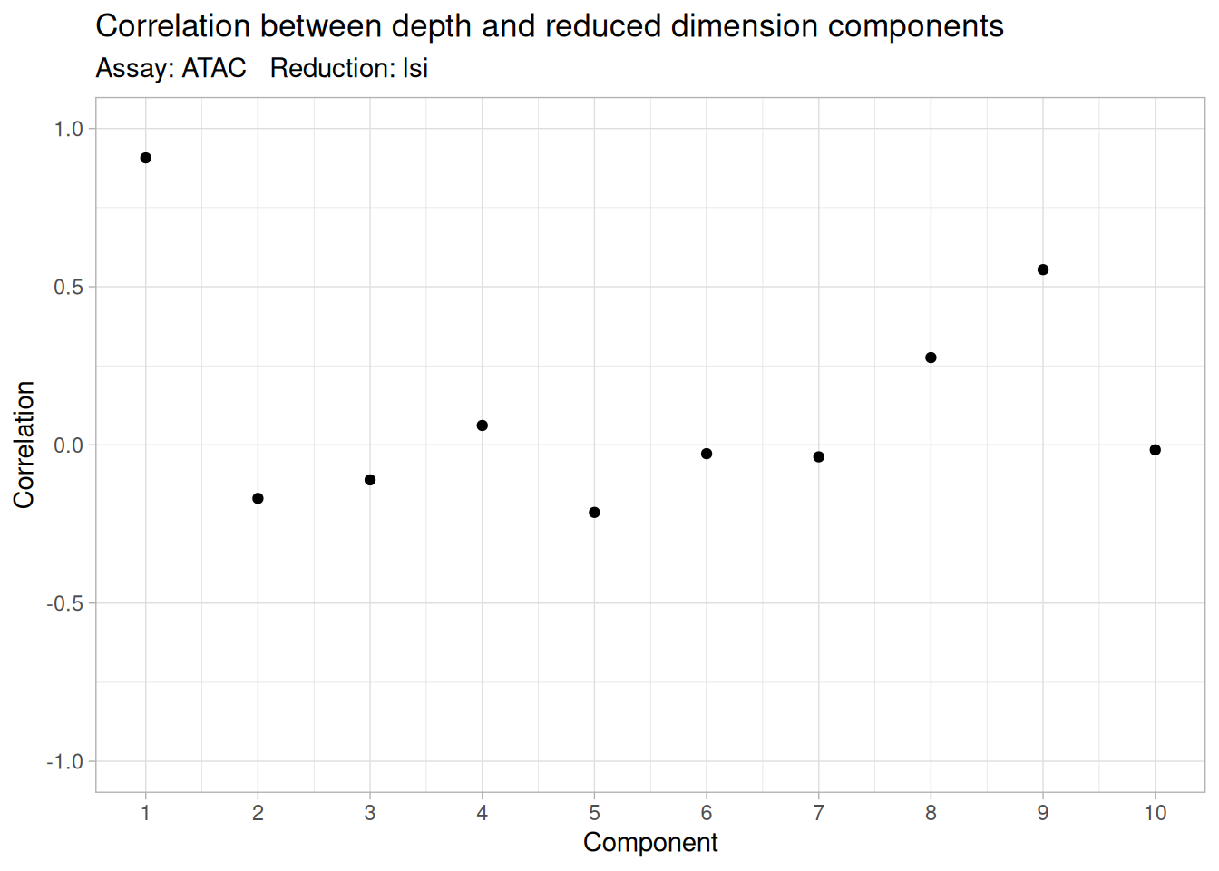

Correlation between each LSI component and the total ATAC fragment count per cell. The first component is almost perfectly correlated with sequencing depth — a technical artifact, not biology — which is why we exclude it from every downstream step and use components 2 onward. The later components show little correlation with depth and are the ones carrying the cell-type signal.

39.7 A joint embedding with weighted nearest neighbors

Here is the heart of vertical integration. We have two reductions of the same cells — a PCA from RNA and an LSI from ATAC — and we want one representation that uses both. The naive approach (just glue the two sets of components together) treats every cell as trusting both modalities equally. But that is rarely true: for some cells the RNA cleanly says “T cell” while the ATAC is murky, and for others the reverse.

Weighted nearest neighbors (WNN) (Hao et al. 2021) handles exactly this by letting every cell weight the two modalities for itself. The intuition is a panel of two advisors. Suppose you must sort people into groups by similarity, and you have two advisors: one judges by what people say (RNA), the other by what they are poised to do (ATAC). For some people the first advisor is far more reliable; for others, the second. The sensible strategy is to ask, for each person individually, which advisor’s notion of “similar people” better matches that person — and to trust that advisor more for that person.

That is essentially WNN’s algorithm. For each cell it asks: using this cell’s RNA neighbors, how well can I reconstruct the cell’s own RNA profile — and using its ATAC neighbors, how well can I reconstruct its own ATAC profile? Whichever modality predicts the cell better earns a higher weight for that cell. These per-cell weights (a number between 0 and 1 for each modality, the two summing to 1) then merge the two neighbor graphs into a single weighted nearest-neighbor graph, which we embed with UMAP and cluster exactly as we would a single-modality graph.

pbmc <- FindMultiModalNeighbors(
  pbmc,
  reduction.list = list("pca", "lsi"),
  dims.list = list(1:50, 2:40),        # RNA PCA 1:50; ATAC LSI drops component 1
  modality.weight.name = "RNA.weight"
)

Calculating cell-specific modality weights

Finding 20 nearest neighbors for each modality.

Calculating kernel bandwidths

Warning in FindMultiModalNeighbors(pbmc, reduction.list = list("pca", "lsi"), :
The number of provided modality.weight.name is not equal to the number of
modalities. RNA.weight ATAC.weight are used to store the modality weights

Finding multimodal neighbors

Constructing multimodal KNN graph

Constructing multimodal SNN graph

pbmc <- RunUMAP(pbmc, nn.name = "weighted.nn", assay = "RNA", reduction.name = "wnn.umap")

Warning: The default method for RunUMAP has changed from calling Python UMAP via reticulate to the R-native UWOT using the cosine metric
To use Python UMAP via reticulate, set umap.method to 'umap-learn' and metric to 'correlation'
This message will be shown once per session

15:46:33 UMAP embedding parameters a = 0.9922 b = 1.112

15:46:34 Commencing smooth kNN distance calibration using 1 thread with target n_neighbors = 20
15:46:36 Found 3 connected components, falling back to random initialization
15:46:36 Initializing from uniform random
15:46:36 Commencing optimization for 200 epochs, with 292842 positive edges
15:46:36 Using rng type: pcg
15:46:39 Optimization finished

pbmc <- FindClusters(pbmc, graph.name = "wsnn", algorithm = 3, resolution = 0.8)

Modularity Optimizer version 1.3.0 by Ludo Waltman and Nees Jan van Eck

Number of nodes: 10032
Number of edges: 374830

Running smart local moving algorithm...
Maximum modularity in 10 random starts: 0.9056
Number of communities: 20
Elapsed time: 4 seconds

39.7.1 What did the joint view buy us?

The payoff is clearest when we put all three embeddings side by side — RNA alone, ATAC alone, and the WNN joint view — and look for cell populations that one modality blurs but the other (and so the joint view) resolves:

pbmc <- RunUMAP(pbmc, reduction = "pca", dims = 1:50, reduction.name = "rna.umap")

15:46:44 UMAP embedding parameters a = 0.9922 b = 1.112

15:46:44 Read 10032 rows and found 50 numeric columns

15:46:44 Using Annoy for neighbor search, n_neighbors = 30

15:46:44 Building Annoy index with metric = cosine, n_trees = 50

0%   10   20   30   40   50   60   70   80   90   100%

[----|----|----|----|----|----|----|----|----|----|

**************************************************|
15:46:45 Writing NN index file to temp file /tmp/RtmpXrGGdm/file5760f50440
15:46:45 Searching Annoy index using 1 thread, search_k = 3000
15:46:48 Annoy recall = 100%
15:46:48 Commencing smooth kNN distance calibration using 1 thread with target n_neighbors = 30
15:46:50 Found 2 connected components, falling back to 'spca' initialization with init_sdev = 1
15:46:50 Using 'irlba' for PCA
15:46:50 PCA: 2 components explained 51.63% variance
15:46:50 Scaling init to sdev = 1
15:46:50 Commencing optimization for 200 epochs, with 447124 positive edges
15:46:50 Using rng type: pcg
15:46:54 Optimization finished

pbmc <- RunUMAP(pbmc, reduction = "lsi", dims = 2:40, reduction.name = "atac.umap")

15:46:54 UMAP embedding parameters a = 0.9922 b = 1.112
15:46:54 Read 10032 rows and found 39 numeric columns
15:46:54 Using Annoy for neighbor search, n_neighbors = 30
15:46:54 Building Annoy index with metric = cosine, n_trees = 50
0%   10   20   30   40   50   60   70   80   90   100%
[----|----|----|----|----|----|----|----|----|----|
**************************************************|
15:46:55 Writing NN index file to temp file /tmp/RtmpXrGGdm/file571052de
15:46:55 Searching Annoy index using 1 thread, search_k = 3000
15:46:57 Annoy recall = 100%
15:46:58 Commencing smooth kNN distance calibration using 1 thread with target n_neighbors = 30
15:47:00 Initializing from normalized Laplacian + noise (using RSpectra)
15:47:00 Commencing optimization for 200 epochs, with 393226 positive edges
15:47:00 Using rng type: pcg
15:47:04 Optimization finished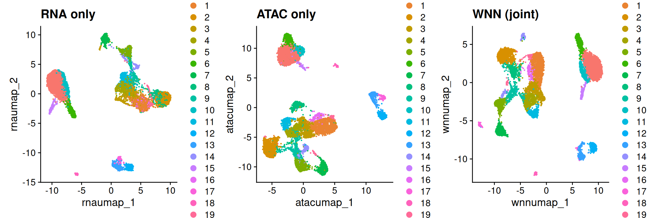

p1 <- DimPlot(pbmc, reduction = "rna.umap")  + ggtitle("RNA only")
p2 <- DimPlot(pbmc, reduction = "atac.umap") + ggtitle("ATAC only")
p3 <- DimPlot(pbmc, reduction = "wnn.umap")  + ggtitle("WNN (joint)")
p1 + p2 + p3

The same PBMCs embedded three ways; every point is a cell, colored by its WNN joint cluster. Left (RNA only): UMAP from gene expression alone. Middle (ATAC only): UMAP from chromatin accessibility alone — typically blurrier, because the near-binary ATAC signal carries less information per cell than expression does. Right (WNN, joint): the embedding that weights both modalities per cell. Read the figure by following one color across the three panels: a cluster that is smeared or split in a single-modality panel but compact and cleanly separated in the joint panel is a population the joint view resolves better than either modality alone. Because the points are colored by the joint clusters, the right-hand panel is the one in which they should look tightest and best separated.

We can also look directly at what WNN learned — the per-cell modality weights. Each cell received an RNA weight (and an ATAC weight equal to 1 − the RNA weight); plotting the RNA weight by cluster shows which cell types lean on expression and which lean on accessibility to define themselves:

VlnPlot(pbmc, features = "RNA.weight", group.by = "seurat_clusters", pt.size = 0)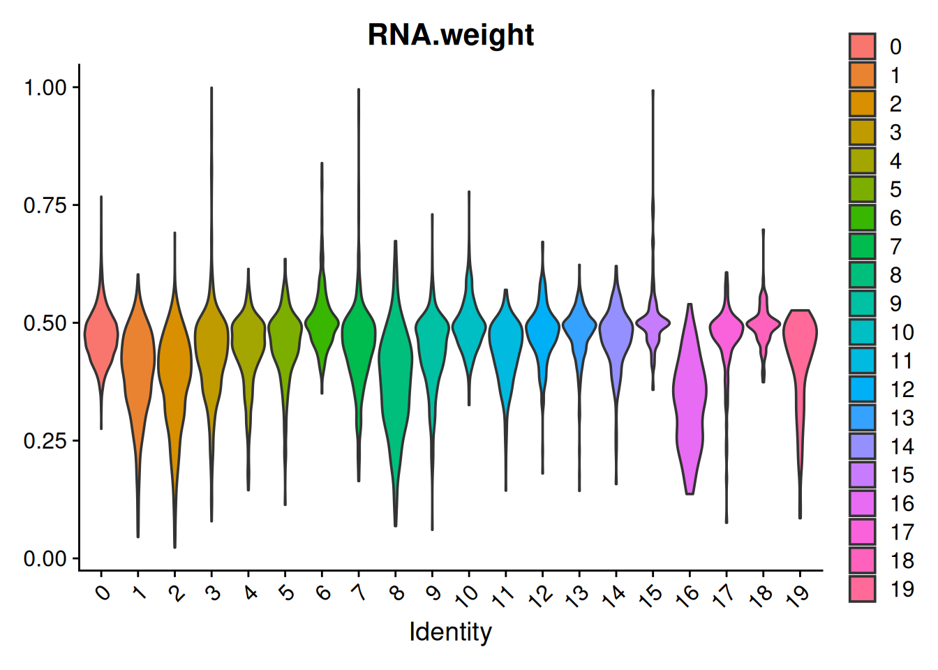

Per-cell RNA modality weight, grouped by WNN cluster. A value near 1 means WNN found that cell’s identity better defined by gene expression; a low value means chromatin accessibility was the more informative modality for that cell. Clusters sitting well above 0.5 are ‘RNA-driven’; those below are ‘ATAC-driven.’ The differences between clusters are the biological readout — they tell you which populations are distinguished more by what they transcribe versus how their chromatin is configured.

39.8 Downstream: linking a peak to the gene it regulates

The unique payoff of paired data is that we can connect a specific open region to a specific gene’s expression in the same cells. The honest, transparent way to see the idea is to compute it by hand for one locus: take a cell-type marker gene, find the accessible peaks near it, and ask whether a peak’s accessibility tracks the gene’s expression across cells. A peak that does is a candidate regulatory element for that gene.

We’ll use MS4A1 (CD20), a canonical B-cell marker. The logic is three steps: find the gene, find the peaks near it, then correlate.

Step 1 — locate the gene. We pull MS4A1’s coordinates from an Ensembl annotation and relabel its chromosome in the chr11 (UCSC) style the ATAC peaks use, then widen to a ±100 kb window — wide enough to catch enhancers, which often sit well outside the gene body. One wrinkle: many gene symbols match two rows in Ensembl — the real protein_coding gene plus an LRG_gene curated-reference duplicate at the same locus. We keep only the protein-coding row so every peak is counted once:

library(EnsDb.Hsapiens.v86)

gene <- "MS4A1"
all.genes <- genes(EnsDb.Hsapiens.v86)              # every gene, as a GRanges
gene.gr   <- all.genes[all.genes$gene_name == gene &
                       all.genes$gene_biotype == "protein_coding"] # one row
seqlevelsStyle(gene.gr) <- "UCSC"                   # "11" -> "chr11"

Warning in (function (seqlevels, genome, new_style) : cannot switch some
GRCh38's seqlevels from NCBI to UCSC style

window <- resize(gene.gr, width = width(gene.gr) + 2e5, fix = "center")
window

GRanges object with 1 range and 6 metadata columns:
                  seqnames            ranges strand |         gene_id
                     <Rle>         <IRanges>  <Rle> |     <character>
  ENSG00000156738    chr11 60355752-60570760      + | ENSG00000156738
                    gene_name   gene_biotype seq_coord_system      symbol
                  <character>    <character>      <character> <character>
  ENSG00000156738       MS4A1 protein_coding       chromosome       MS4A1
                  entrezid
                    <list>
  ENSG00000156738      931
  -------
  seqinfo: 357 sequences (1 circular) from 2 genomes (hg38, GRCh38)

Step 2 — find nearby peaks. The ChromatinAssay carries each peak’s coordinates, so we ask which peaks fall inside the window. We index back into the assay’s own peak names so the identifiers match exactly:

peak.gr  <- granges(pbmc[["ATAC"]])
idx      <- queryHits(findOverlaps(peak.gr, window))
peak.ids <- rownames(pbmc[["ATAC"]])[idx]
length(peak.ids)                                    # how many peaks sit near MS4A1?

[1] 23

Step 3 — correlate accessibility with expression. For each nearby peak we compute the Spearman correlation, across all 10,032 cells, between that peak’s accessibility and MS4A1’s expression. A peak whose opening rises and falls with the gene’s expression is a candidate regulatory element for it:

acc  <- GetAssayData(pbmc, assay = "ATAC", layer = "data")[peak.ids, , drop = FALSE]
expr <- GetAssayData(pbmc, assay = "RNA",  layer = "data")[gene, ]

peak.cor <- apply(acc, 1, function(a) cor(a, expr, method = "spearman"))
sort(peak.cor, decreasing = TRUE)[1:10]             # the top candidate links

chr11-60455290-60456088 chr11-60498212-60499391 chr11-60476867-60477719 
              0.5861696               0.3864819               0.3556311 
chr11-60457557-60458006 chr11-60485853-60486383 chr11-60357719-60358258 
              0.2812676               0.2474239               0.1842331 
chr11-60396248-60397424 chr11-60459521-60459691 chr11-60376380-60382255 
              0.1827865               0.1327127               0.1218045 
chr11-60366868-60368023 
              0.1187863 

The most strongly correlated peak is typically the gene’s own promoter; the others are candidate enhancers that open in the same cells that express MS4A1 — precisely the sort of regulatory link that only paired measurement, in the same cells, can reveal.

A correlation coefficient is a single number; it helps to see what it summarizes. Below we plot, cell by cell, MS4A1 expression against accessibility — for the promoter peak (the strongest link) and, for contrast, a nearby peak whose accessibility is essentially uncorrelated with expression. Single-cell data are sparse, so most cells register neither signal and pile up at the origin; rather than overplot ~10,000 semi-transparent points we bin them into a 2-D histogram with a log-scaled colour:

library(ggplot2)
library(patchwork)

top.peak  <- names(sort(peak.cor, decreasing = TRUE))[1] # strongest link (promoter)
null.peak <- names(peak.cor)[which.min(abs(peak.cor))]   # nearby peak, no link

link_panel <- function(peak, tag) {
  df <- data.frame(accessibility = acc[peak, ], expression = expr)
  ggplot(df, aes(accessibility, expression)) +
    geom_bin2d(bins = 40) +
    scale_fill_viridis_c(trans = "log10", name = "cells") +
    labs(title = tag,
         subtitle = sprintf("%s  (Spearman ρ = %.2f)", peak, peak.cor[peak]),
         x = "ATAC accessibility (TF-IDF)",
         y = "MS4A1 expression (log-normalised)") +
    theme_minimal(base_size = 10)
}

link_panel(top.peak,  "Promoter: accessibility tracks expression") +
  link_panel(null.peak, "Nearby peak: no link")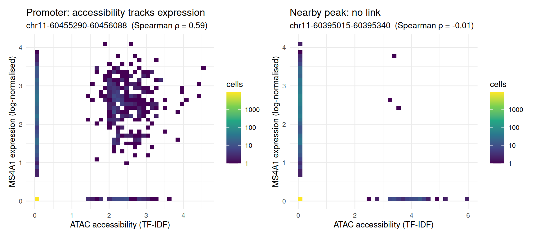

Per-cell ATAC accessibility (x) versus MS4A1 expression (y) across all 10,032 cells, binned into a 2-D histogram with a log-scaled colour. Left — the promoter peak: a distinct population of cells (the B cells) is high in both modalities, and it is this joint high–high cloud that drives the positive Spearman correlation. Right — a nearby peak with ρ ≈ 0: the accessible cells (spread along the x-axis at zero expression) and the expressing cells (spread up the y-axis at zero accessibility) are largely different cells, so the two signals never coincide. The bright bin at the origin is the majority of cells in which neither modality was detected — the pervasive dropout of single-cell assays, and the reason a density view is clearer here than a raw scatterplot.

TipWhere this goes next

Production tools formalize this step: Signac::LinkPeaks() adds GC-content and background correction (at the cost of a BSgenome and the fragment file), and full gene-regulatory-network methods (SCENIC+, Pando) chain peak→gene links with transcription-factor motifs to reconstruct regulatory circuits. We compute the bare correlation here so the concept is unmistakable.

39.9 Summary

• RNA and ATAC are complementary: expression is the output, accessibility is the regulatory wiring — and a cell can open a locus before it transcribes the gene.
• Know your integration shape first. This was a vertical problem: a multiome assay handed us the cell correspondence, so the task was to combine two views, not to match cells.
• The two modalities live in different feature spaces (genes vs. peaks), and the sparse, near-binary ATAC matrix needs TF-IDF + LSI, not the log-PCA recipe used for RNA — and its first LSI component usually encodes depth, not biology.
• WNN builds a single embedding by learning, per cell, how much to trust each modality — recovering structure that either modality alone can blur.
• Paired data uniquely lets you link peaks to genes in the same cells, the first step toward reconstructing regulatory logic.

39.10 What’s next: the unpaired case

This chapter handled the vertical problem, where the multiome assay handed us the cell correspondence for free. The harder and very common case is diagonal integration — a separate scRNA dataset and scATAC dataset with no shared cells — where we must infer the correspondence ourselves. The next chapter tackles it with anchor-based label transfer, and uses a clever trick: we take this very multiome dataset, throw away the pairing, and try to recover it — giving us a known ground truth to grade the integration against.

Argelaguet, Ricard, Anna S. E. Cuomo, Oliver Stegle, and John C. Marioni. 2021. “Computational Principles and Challenges in Single-Cell Data Integration.” Nature Biotechnology 39 (10): 1202–15. https://doi.org/10.1038/s41587-021-00895-7.

Cusanovich, Darren A., Riza Daza, Andrew Adey, et al. 2015. “Multiplex Single-Cell Profiling of Chromatin Accessibility by Combinatorial Cellular Indexing.” Science 348 (6237): 910–14. https://doi.org/10.1126/science.aab1601.

Eckenrode, Kelly B., Dario Righelli, Marcel Ramos, et al. 2023. “Curated Single Cell Multimodal Landmark Datasets for R/Bioconductor.” PLOS Computational Biology 19 (8): e1011324. https://doi.org/10.1371/journal.pcbi.1011324.

Hao, Yuhan, Stephanie Hao, Erica Andersen-Nissen, et al. 2021. “Integrated Analysis of Multimodal Single-Cell Data.” Cell 184 (13): 3573–3587.e29. https://doi.org/10.1016/j.cell.2021.04.048.

Schep, Alicia N., Beijing Wu, Jason D. Buenrostro, and William J. Greenleaf. 2017. “chromVAR: Inferring Transcription-Factor-Associated Accessibility from Single-Cell Epigenomic Data.” Nature Methods 14 (10): 975–78. https://doi.org/10.1038/nmeth.4401.

Stuart, Tim, Avi Srivastava, Shaista Madad, Caleb A. Lareau, and Rahul Satija. 2021. “Single-Cell Chromatin State Analysis with Signac.” Nature Methods 18 (11): 1333–41. https://doi.org/10.1038/s41592-021-01282-5.

Vandereyken, Katy, Alejandro Sifrim, Bernard Thienpont, and Thierry Voet. 2023. “Methods and Applications for Single-Cell and Spatial Multi-Omics.” Nature Reviews Genetics 24 (8): 494–515. https://doi.org/10.1038/s41576-023-00580-2.