22 Worked example: classifying cancer types from gene expression

Author

Affiliation

University of Colorado
Anschutz School of Medicine

Published

June 1, 2024

Modified

June 2, 2026

The earlier machine learning chapters introduced the ideas: the difference between supervised and unsupervised learning (Introduction), the workhorse algorithms (Supervised Learning), and the mlr3 framework that wraps all of them in one tidy interface (The mlr3verse). This is the first of three chapters where those ideas meet real data.

Here we tackle a classification problem: given a tumour’s gene-expression profile, can we predict which cancer type it is? This is the first of three worked examples — the next two predict age from DNA methylation and gene expression from histone marks — and because it comes first, it also lays down the habits the others reuse: how to set up an mlr3 analysis, how to split the data, how to select features, and how to read the results without fooling yourself.

Three ideas from the introduction do the heavy lifting in every one of these examples, so it is worth stating them plainly here, in the concrete terms of gene-expression classification:

Feature selection. A tumour profile measures tens of thousands of genes, but most of them barely change from one sample to the next. A gene that stays flat across every tumour cannot help tell cancer types apart — it is noise. So we select the genes that vary the most and discard the rest, shrinking the problem to the handful of features that actually carry signal.
The train/test split. We hold back a slice of tumours that the model never sees while it learns. Scoring it on those unseen tumours is the only honest estimate of how it will classify a new patient’s biopsy — the thing we actually care about.
Overfitting. A model given too much freedom — a decision tree grown too deep, say — can memorize the exact training tumours instead of learning a rule that generalizes. We catch this by watching the gap between the training score and the test score.

The next two chapters revisit all three from different biological angles; this is where we meet them as first principles.

The through-line for all three worked examples

Feature selection, an honest train/test split, and vigilance against overfitting are the spine of every worked example. Here they take their plainest form: keep the most variable genes, hold out some tumours, and distrust a model that aces the training set but stumbles on the test set. Hold on to this picture — the methylation and histone-mark chapters return to each idea and add a new twist.

22.1 What you’ll learn

Turn a real genomics dataset into an mlr3 task with as_task_classif().
Split data into training and test sets, and explain why that split protects you from fooling yourself.
Select features by variance, and say why selection must happen on the training data only.
Train and predict with several learners — kNN, a classification tree, and a random forest — using the same handful of mlr3 calls.
Interpret a confusion matrix and an accuracy, and recognize overfitting when the test score falls below the training score.

22.2 A quick recap of the mlr3 workflow

You met the mlr3 building blocks in The mlr3verse; here is the one-paragraph reminder so you can keep your eyes on the biology. Every analysis in these worked-example chapters follows the same four-step rhythm (Figure 22.1):

Task — bundle your data with the name of the column you want to predict (the target). Classification tasks predict a category; regression tasks predict a number.
Learner — pick an algorithm by name with lrn(), e.g. lrn("classif.kknn").
Train and predict — call learner$train(task, ...) then learner$predict(task, ...).
Measure — score the predictions with msrs(), e.g. accuracy for classification or R² for regression.

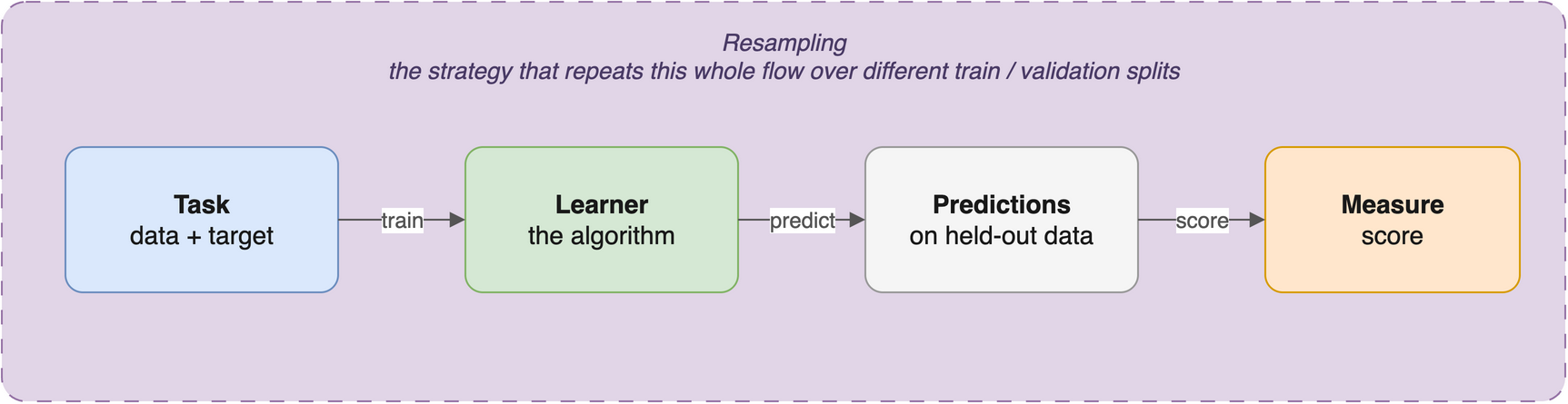
Figure 22.1: The mlr3 ecosystem. A consistent set of objects — tasks, learners, measures, and resampling strategies — that snap together the same way for every algorithm.

The power of mlr3 is that this rhythm is identical no matter which algorithm you use. Swapping a k-nearest-neighbours model for a random forest is a one-line change to the lrn() call; everything else stays the same. For the full tour of tasks, learners, measures, and resamplings, see The mlr3verse; the official mlr3 book is the deep reference.

The single most important habit: split your data

A model that is tested on the same data it was trained on will look far better than it really is — it can simply memorize the answers. We always hold out a test set that the model never sees during training, and we report performance from that held-out set. This is the only honest estimate of how the model will behave on new patients or new genes.

22.3 Setup

library(mlr3verse)
library(GEOquery)
library(mlr3learners) # for knn
library(ranger)       # for random forests
set.seed(789)

22.4 Understanding the problem

In this example we classify cancer types from gene-expression data. The data come from Brouwer-Visser et al. (2018), available through the Gene Expression Omnibus (GEO), a public repository of functional-genomics data. The study profiled gene expression in tumours of several types, and our question is: given a tumour’s expression profile, can we predict which cancer type it is?

Before building anything, it pays to answer four questions about the task:

What are the features? The expression level of each gene.
What is the target? The cancer type (a category).
What kind of task is this? Classification — we are predicting a label, not a number.
What is the goal? A model that assigns the correct cancer type to a tumour it has never seen.

22.5 Data preparation

We use the GEOquery package to fetch dataset GSE103512. This downloads over the network, so give it a moment.

gse <- getGEO("GSE103512")[[1]]

GEOquery was written in 2007 and returns an older Bioconductor structure, the ExpressionSet. As a first housekeeping step we convert it to the modern SummarizedExperiment (covered in the SummarizedExperiment chapter).

library(SummarizedExperiment)
se <- as(gse, "SummarizedExperiment")

Let’s look at two variables of interest: the cancer type and whether each sample is tumour or normal tissue.

with(colData(se), table(`cancer.type.ch1`, `normal.ch1`))

               normal.ch1
cancer.type.ch1 no yes
          BC    65  10
          CRC   57  12
          NSCLC 60   9
          PCA   60   7

This table tells us how many samples we have of each cancer type, split by tumour versus normal status. Most samples are tumours (normal: no), with a smaller set of matched normal tissues. We’ll keep only the tumour samples for classification.

Always explore before you model

Missing values, outliers, and unexpected categories can quietly break a machine learning model. Plots, summaries, PCA, and clustering all help you understand the data first. Time spent here saves time later — and saves you from confidently reporting a result that was an artifact all along.

22.6 Feature selection and data cleaning

This dataset measures thousands of genes, but most of them barely change between samples and carry little signal. We will keep the 200 genes with the highest variance across samples, on the reasoning that a gene that never changes can’t help us tell cancer types apart. (Other selection strategies exist, such as ranking genes by their correlation with the outcome.)

Select features on the training data only

In a fully rigorous workflow, feature selection must use the training data only — never the test data. If you peek at the test data while choosing features, information leaks across the split and your test score is no longer honest. (For simplicity this example selects on the full matrix; in a real analysis, fold the selection step inside the training split.)

The apply() function applies a function to each row or column of a matrix. Here we apply sd() (standard deviation) to each row of the expression matrix to get a vector of per-gene variability, then keep the 200 most variable genes among the tumour samples.

sds <- apply(assay(se, 'exprs'), 1, sd)
## keep the 200 most-variable genes, tumour samples only
se_small <- se[order(sds, decreasing = TRUE)[1:200],
               colData(se)$characteristics_ch1.1 == 'normal: no']
# remove genes with no gene symbol
se_small <- se_small[rowData(se_small)$Gene.Symbol != '', ]

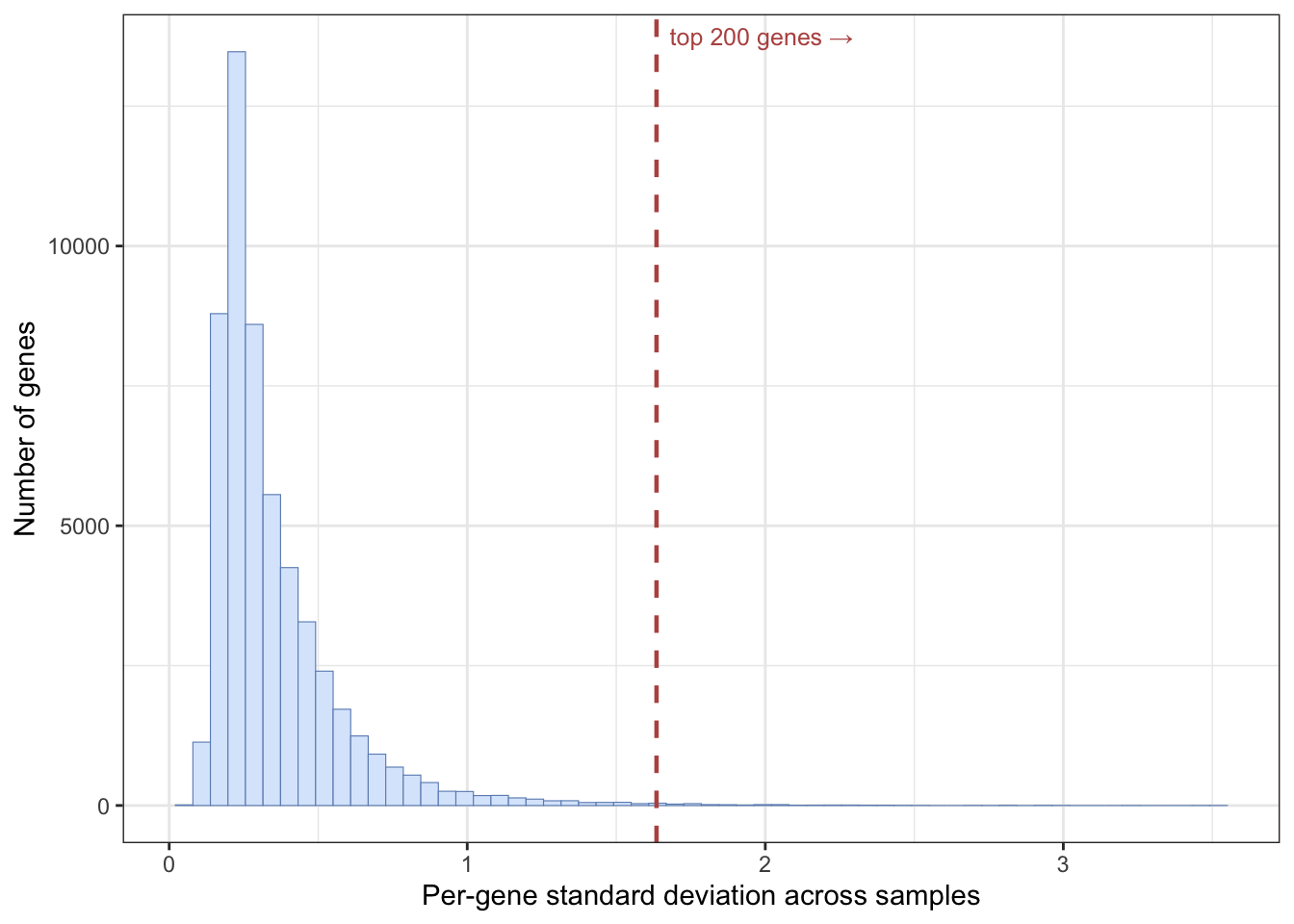
To make the data easier to work with, we use one of the rowData columns (the gene symbol) as the row names. make.names() ensures those names are valid, unique R variable names.

## convert to a matrix for later use
expr_mat <- assay(se_small, 'exprs')
rownames(expr_mat) <- make.names(rowData(se_small)$Gene.Symbol)

mlr3 expects samples in rows and features in columns, so we transpose the matrix and attach the cancer type as a column.

feat_dat <- t(expr_mat)
tumor <- data.frame(tumor_type = colData(se_small)$cancer.type.ch1, feat_dat)

This is another good moment to check the data: confirm the dimensions, the column names, and the data types are what you expect before moving on.

22.7 Creating the task

The first mlr3 step is to create a task — a dataset paired with the name of the target column. Because the target (cancer type) is a category, this is a classification task, so we use as_task_classif(). The target must be a factor.

tumor$tumor_type <- as.factor(tumor$tumor_type)
task <- as_task_classif(tumor, target = 'tumor_type')

22.8 Splitting the data

We randomly assign two-thirds of the samples to a training set and one-third to a test set. The model learns from the training set; we judge it on the test set it never saw. We seed the split so the result is reproducible.

set.seed(7)
train_set <- sample(task$row_ids, 0.67 * task$nrow)
test_set <- setdiff(task$row_ids, train_set)

In the next sections we train three different learners on this task — k-nearest-neighbours, a classification tree, and a random forest — and compare how each one does at predicting cancer type.

22.9 k-nearest-neighbours

The first learner is k-nearest-neighbours (kNN). Its idea is simple: a new sample is classified by looking at the k most similar samples and taking a vote. The number of neighbours, k, is a tunable setting; we’ll use the default of 7. (mlr3 can tune such settings automatically, but that’s beyond this chapter.)

22.9.1 Create the learner

In mlr3 an algorithm is a learner, created with lrn() by name.

learner <- lrn("classif.kknn")

Calling lrn() with no arguments lists every available learner.

lrn()

<DictionaryLearner> with 55 stored values
Keys: classif.cv_glmnet, classif.debug, classif.featureless,
  classif.glmnet, classif.kknn, classif.lda, classif.log_reg,
  classif.multinom, classif.naive_bayes, classif.nnet, classif.qda,
  classif.ranger, classif.rpart, classif.svm, classif.xgboost,
  clust.agnes, clust.ap, clust.bico, clust.birch, clust.clara,
  clust.cmeans, clust.cobweb, clust.dbscan, clust.dbscan_fpc,
  clust.diana, clust.em, clust.fanny, clust.featureless, clust.ff,
  clust.hclust, clust.hdbscan, clust.kkmeans, clust.kmeans,
  clust.kproto, clust.MBatchKMeans, clust.mclust, clust.meanshift,
  clust.optics, clust.pam, clust.protoclust, clust.SimpleKMeans,
  clust.specc, clust.xmeans, regr.cv_glmnet, regr.debug,
  regr.featureless, regr.glmnet, regr.kknn, regr.km, regr.lm,
  regr.nnet, regr.ranger, regr.rpart, regr.svm, regr.xgboost

22.9.2 Train

learner$train() takes the task and the row IDs of the training data.

learner$train(task, row_ids = train_set)

We could inspect the trained model, but for kNN the printout is large, so this chunk is left for you to run on your own.

# output is large, so do this on your own
learner$model

22.9.3 Predict

Let’s first predict the classes of the training data. We already know those answers, but predicting on the training set gives us a baseline we can compare against the test set to detect overfitting.

pred_train <- learner$predict(task, row_ids = train_set)

And now the test data — the honest evaluation:

pred_test <- learner$predict(task, row_ids = test_set)

22.9.4 Assess

A confusion matrix cross-tabulates the true class (rows) against the predicted class (columns). Correct predictions land on the diagonal; off-diagonal entries are mistakes.

pred_train$confusion

        truth
response BC CRC NSCLC PCA
   BC    42   0     0   0
   CRC    0  40     0   0
   NSCLC  1   0    44   0
   PCA    0   0     0  35

On the training data, almost every sample falls on the diagonal — the model classifies the data it learned from very well, as expected.

Accuracy summarizes this in one number: the fraction of samples classified correctly.

measures <- msrs(c('classif.acc'))
pred_train$score(measures)

classif.acc 
  0.9938272

Now the test set, which the model never saw during training:

pred_test$confusion

        truth
response BC CRC NSCLC PCA
   BC    22   0     0   0
   CRC    0  17     1   0
   NSCLC  0   0    15   0
   PCA    0   0     0  25

pred_test$score(measures)

classif.acc 
     0.9875

The test accuracy is the number to trust. If it is noticeably lower than the training accuracy, the model has overfit — it memorized the training samples rather than learning a rule that generalizes. Compare the two numbers above: how big is the gap?

22.10 Classification tree

A classification tree asks a series of yes/no questions about the features — for example, “is gene X expressed above some threshold?” — and follows the answers down branches to a predicted class. At each split it picks the feature that best separates the classes, and it keeps splitting until the groups are reasonably pure. Trees are appealing because you can read them.

22.10.1 Train

We set keep_model = TRUE so we can inspect the fitted tree afterwards.

learner <- lrn("classif.rpart", keep_model = TRUE)
learner$train(task, row_ids = train_set)

Here is the trained model:

learner$model

n= 162 

node), split, n, loss, yval, (yprob)
      * denotes terminal node

 1) root 162 118 NSCLC (0.26543210 0.24691358 0.27160494 0.21604938)  
   2) CDHR5>=5.101625 40   0 CRC (0.00000000 1.00000000 0.00000000 0.00000000) *
   3) CDHR5< 5.101625 122  78 NSCLC (0.35245902 0.00000000 0.36065574 0.28688525)  
     6) ACPP< 6.088431 87  43 NSCLC (0.49425287 0.00000000 0.50574713 0.00000000)  
      12) GATA3>=4.697803 41   1 BC (0.97560976 0.00000000 0.02439024 0.00000000) *
      13) GATA3< 4.697803 46   3 NSCLC (0.06521739 0.00000000 0.93478261 0.00000000) *
     7) ACPP>=6.088431 35   0 PCA (0.00000000 0.00000000 0.00000000 1.00000000) *

Trees are easy to visualize when they are small. This one has only a couple of splits, which makes the decision logic easy to follow.

library(mlr3viz)
library(ggparty)

Loading required package: ggplot2

Loading required package: partykit

Loading required package: grid

Loading required package: libcoin

Loading required package: mvtnorm


Attaching package: 'partykit'

The following object is masked from 'package:SummarizedExperiment':

    width

The following object is masked from 'package:GenomicRanges':

    width

The following object is masked from 'package:IRanges':

    width

The following object is masked from 'package:S4Vectors':

    width

The following object is masked from 'package:BiocGenerics':

    width

autoplot(learner, type = 'ggparty')

Warning in ggparty::geom_edge_label(): Ignoring unknown parameters:
`label.size`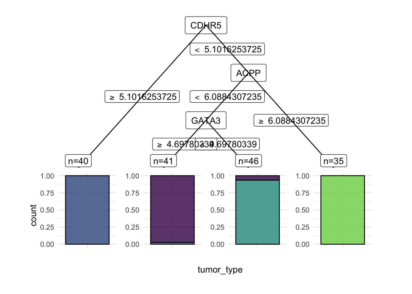

22.10.2 Predict

As before, we predict on both the training and test sets.

pred_train <- learner$predict(task, row_ids = train_set)
pred_test <- learner$predict(task, row_ids = test_set)

22.10.3 Assess

Important

Performance should always be reported from an independent test set, never from the training set.

pred_train$confusion

        truth
response BC CRC NSCLC PCA
   BC    40   0     1   0
   CRC    0  40     0   0
   NSCLC  3   0    43   0
   PCA    0   0     0  35

measures <- msrs(c('classif.acc'))
pred_train$score(measures)

classif.acc 
  0.9753086

pred_test$confusion

        truth
response BC CRC NSCLC PCA
   BC    20   0     1   0
   CRC    0  17     3   0
   NSCLC  2   0    12   0
   PCA    0   0     0  25

pred_test$score(measures)

classif.acc 
      0.925

A single tree is a simple model, so it often classifies the training data less perfectly than kNN did, but it may generalize about as well to the test set. Look at the test accuracy and the test confusion matrix: which cancer types does the tree confuse with each other?

Overfitting

When the test score is much worse than the training score, the model is likely overfit — it has learned the training data’s quirks rather than a general rule. How you fix overfitting depends on the model (simpler trees, more regularization, more data), but a large train/test gap is always a signal to look more carefully at model choice and settings.

22.11 Random forest

A random forest grows many decision trees, each on a random subset of the data and features, and averages their votes. Because the trees disagree in different ways, their combined prediction is usually more accurate and more stable than any single tree. We set importance = "impurity" so the model also reports how useful each gene was.

22.11.1 Train

set.seed(789)
learner <- lrn("classif.ranger", importance = "impurity")
learner$train(task, row_ids = train_set)

We can look at the fitted forest:

learner$model

Ranger result

Call:
 ranger::ranger(dependent.variable.name = task$target_names, data = task$data(),      probability = self$predict_type == "prob", importance = "impurity",      num.threads = 1L) 

Type:                             Classification 
Number of trees:                  500 
Sample size:                      162 
Number of independent variables:  192 
Mtry:                             13 
Target node size:                 1 
Variable importance mode:         impurity 
Splitrule:                        gini 
OOB prediction error:             0.00 %

The printout reports an OOB (out-of-bag) error. Because each tree is trained on a bootstrap sample, the samples it didn’t see act as a free held-out set; the OOB error estimates test performance without needing a separate split. A low OOB error is a good sign.

Random forests also give us a variable importance score — roughly, how often and how usefully each gene was used across the trees.

head(learner$importance(), 15)

    CDHR5     FABP1     KRT20     GATA3    LGALS4     TRPS1   SFTPB.1     EFHD1 
 4.668165  4.042106  3.722492  3.470107  3.271688  3.047672  2.925743  2.895864 
   EPS8L3   TRPS1.1   GATA3.1 SLC45A3.1    TSPAN8    KLK3.1     AZGP1 
 2.894204  2.442827  2.432394  2.242252  2.163998  2.134062  2.119718

The most important genes here are the ones the forest leaned on most heavily to separate the cancer types. It’s worth looking a few of them up to see whether they make biological sense — and comparing them to the gene the single tree split on.

22.11.2 Predict and assess

pred_train <- learner$predict(task, row_ids = train_set)
pred_test <- learner$predict(task, row_ids = test_set)

pred_train$confusion

        truth
response BC CRC NSCLC PCA
   BC    43   0     0   0
   CRC    0  40     0   0
   NSCLC  0   0    44   0
   PCA    0   0     0  35

measures <- msrs(c('classif.acc'))
pred_train$score(measures)

classif.acc 
          1

pred_test$confusion

        truth
response BC CRC NSCLC PCA
   BC    22   0     0   0
   CRC    0  17     0   0
   NSCLC  0   0    16   0
   PCA    0   0     0  25

pred_test$score(measures)

classif.acc 
          1

Compare all three test accuracies — kNN, the single tree, and the random forest. On most genomics classification problems the random forest is the strongest of the three, and it gives you the importance ranking as a bonus.

22.12 Summary

You have now run a complete classification analysis on real gene-expression data, all through the mlr3 workflow:

You turned a GEO dataset into an mlr3 classification task, split it into training and test sets, and selected the 200 most-variable genes as features.
You trained three learners — kNN, a single classification tree, and a random forest — and read each one’s confusion matrix and accuracy.
On most genomics classification problems the random forest is the strongest of the three, and it hands you a gene-importance ranking for free.

The disciplines you practised here recur in every analysis: split the data, select features thoughtfully, train then predict, and judge every model by its test-set score. That last habit — never trusting the training score — is the single most important thing to carry forward to the next two chapters.

22.13 Exercises

Each exercise reuses objects you already built, so the solutions are quick to run.

Swap a learner. The random forest above used impurity-based importance. Train a support vector machine instead and compare its test accuracy to the random forest. (You may need library(e1071); if it isn’t installed, fall back to comparing kNN with a different k.)
NoteSolution
svm_learner <- lrn("classif.svm") svm_learner$train(task, row_ids = train_set) svm_pred <- svm_learner$predict(task, row_ids = test_set) svm_pred$score(msrs(c('classif.acc')))
The point is that swapping algorithms is a one-line change to lrn() — everything else in the workflow is identical. Compare the test accuracy to the forest’s; on this small, high-variance dataset the ranking can shift, which is why you always judge on the held-out test set.
Change the feature-selection cutoff. We kept the 200 most-variable genes. Conceptually, what would you expect to happen to the random forest’s test accuracy if you kept only the top 50, or the top 1000?

NoteSolution

Too few features (top 50) may discard genes that help separate the rarer cancer types, lowering accuracy. Too many (top 1000) reintroduces low-variance, low-signal genes that add noise and computation without much benefit — and they raise the risk of overfitting. The “right” cutoff is a balance, best chosen by comparing test-set performance across a few values rather than guessing.