18  K-means clustering

Author

Affiliation

Sean Davis

University of Colorado
Anschutz School of Medicine

When yeast cells run low on glucose, they flip their entire metabolic program — switching from fermentation to respiration in an event called the diauxic shift. DeRisi et al. (1997) watched this happen by measuring the expression of roughly 6,400 genes at seven time points across the shift. That leaves you with a wall of numbers: 6,400 genes, each with its own little trajectory over time. Some genes ramp up as the cells switch fuels, some shut down, and most barely move at all. How do you find the groups of genes that rise and fall together — the ones that might be co-regulated, taking part in the same biological response?

That is exactly the kind of question k-means clustering answers. It is an unsupervised method: you don’t tell it which genes belong together, you just ask it to sort the genes into a handful of groups so that genes with similar behavior land in the same group. In this chapter you’ll use k-means on the DeRisi yeast data — the same dataset you met in the SummarizedExperiment chapter — to pull out clusters of co-regulated genes and then read their temporal profiles back as biology.

18.1 What you’ll learn

• Explain in plain language what k-means clustering does and when it’s useful.
• Pull a public dataset from NCBI GEO with getGEO() and convert it to a SummarizedExperiment.
• Filter a gene-expression matrix down to its most variable (most informative) genes using the standard deviation.
• Run kmeans() on real data and make the result reproducible with set.seed().
• Plot each cluster’s expression profile and interpret what the clusters say about the diauxic shift.

18.2 What k-means does

K-means clustering is a method for finding groups in a dataset. It is an unsupervised learning technique: it doesn’t rely on previously labeled data. Instead, it finds structure directly from the data, based on how similar the data points are to one another (Figure 18.1).

Figure 18.1: K-means clustering takes a dataset and divides it into k clusters.

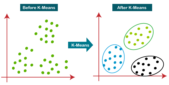
The idea is to split the data into k groups, called clusters, so that each point belongs to the cluster whose average it is closest to. The algorithm tries to make points within a cluster as similar as possible while keeping different clusters as distinct as possible. For our yeast data, a “point” is a single gene, and “similar” means follows a similar expression pattern over the time course.

TipAn analogy for the algorithm

Imagine k party hosts scattered around a room full of guests. Each guest walks to the nearest host (assignment). Each host then moves to the middle of their own group (update). Guests re-check who is now closest and move again, and the hosts re-center. Repeat until nobody needs to move. The final huddles are your clusters, and each host’s position is a centroid — the average of its group.

18.3 The k-means algorithm

Spelled out, k-means follows these steps:

1. Choose the number of clusters, k.
2. Place k centroids at random (often by picking k of the data points).
3. Assign each data point to its nearest centroid.
4. Update each centroid to the mean of the points assigned to it.
5. Repeat steps 3 and 4 until the centroids stop moving (or a maximum number of iterations is reached).

When the centroids stabilize, the algorithm has converged, and the final clusters represent the patterns in the data.

Warningk-means is random — seed it

Step 2 starts from a random placement of centroids, so two runs can give slightly different clusters (and the cluster numbers can be shuffled). Whenever you want a result you can reproduce — and a frozen figure that doesn’t change on every render — call set.seed() before kmeans().

18.4 Pros and cons of k-means clustering

Compared to other clustering algorithms, k-means has several advantages:

• Simplicity — the algorithm is straightforward and easy to implement, even on large datasets.
• Scalability — it adapts well to large datasets with optimization or parallel processing.
• Speed — it is generally fast, especially when k is small.
• Interpretability — the results are easy to read: every point gets a single cluster label.

It also has real limitations:

• Choice of k — you have to pick the number of clusters yourself, and a poor choice gives poor results. Domain knowledge and experimentation help.
• Sensitivity to initial conditions — different random starts can give different answers, which is why you seed and sometimes re-run.
• Assumes round, even clusters — k-means expects roughly spherical, similarly sized clusters, and struggles when the real groups have other shapes.
• Sensitivity to outliers — a few extreme points can drag a centroid around, so cleaning or filtering the data first helps.

Despite these limits, k-means remains a popular, widely used tool for exploring data — and it is especially handy in biology, where spotting groups of co-behaving genes can hint at shared function or regulation.

18.5 A worked example: the diauxic shift

18.5.1 The data and experimental background

The data come from DeRisi et al. (1997). From their abstract:

DNA microarrays containing virtually every gene of Saccharomyces cerevisiae were used to carry out a comprehensive investigation of the temporal program of gene expression accompanying the metabolic shift from fermentation to respiration. The expression profiles observed for genes with known metabolic functions pointed to features of the metabolic reprogramming that occur during the diauxic shift, and the expression patterns of many previously uncharacterized genes provided clues to their possible functions.

These data are available from NCBI GEO as GSE28.

Here is the biology in brief. When baker’s yeast grows on glucose with plenty of oxygen, it still prefers to ferment the glucose rather than respire it — even though respiration is more efficient. Once the glucose runs low, the cells switch metabolic gears to respiration. That switch is the diauxic shift. This experiment profiles about 6,400 genes across a time course spanning the shift.

These data have no replicates; they are a single time course. Watching how groups of genes behave across that course can reveal biology — both about the system and about individual genes. So we’ll use clustering to group genes with similar expression patterns over time, then look at those groups.

Your goal: use kmeans() to divide the most variable (most informative) genes into a few groups, then visualize each group’s temporal profile.

18.5.2 Getting the data

These data were deposited at NCBI GEO back in 2002. GEOquery can pull them out in one call.

library(GEOquery)
gse <- getGEO("GSE28")[[1]]
class(gse)

[1] "ExpressionSet"
attr(,"package")
[1] "Biobase"

GEOquery predates the SummarizedExperiment class, so it hands you an older ExpressionSet. Bioconductor can convert that into the SummarizedExperiment you already know how to work with.

library(SummarizedExperiment)
gse <- as(gse, "SummarizedExperiment")
gse

class: SummarizedExperiment 
dim: 6400 7 
metadata(3): experimentData annotation protocolData
assays(1): exprs
rownames(6400): 1 2 ... 6399 6400
rowData names(20): ID ORF ... FAILED IS_CONTAMINATED
colnames(7): GSM887 GSM888 ... GSM892 GSM893
colData names(33): title geo_accession ... supplementary_file
  data_row_count

A quick look at the sample descriptions in colData() suggests the columns aren’t in time order:

colData(gse)$title

[1] "diauxic shift timecourse: 15.5 hr" "diauxic shift timecourse: 0 hr"   
[3] "diauxic shift timecourse: 18.5 hr" "diauxic shift timecourse: 9.5 hr" 
[5] "diauxic shift timecourse: 11.5 hr" "diauxic shift timecourse: 13.5 hr"
[7] "diauxic shift timecourse: 20.5 hr"

So reorder them by hand so the columns run in time-course order:

gse <- gse[, c(2, 4, 5, 6, 1, 3, 7)]

18.5.3 Preprocessing: keep only the informative genes

Most of those 6,400 genes barely change across the time course. Feeding all of them to the clustering algorithm is slow and, worse, lets thousands of flat, noisy genes drown out the few hundred that actually respond to the diauxic shift.

So before clustering, you filter down to the genes that carry signal. A simple, effective filter is the standard deviation of each gene across the samples: a gene whose expression swings widely over the time course has a high standard deviation, while a gene that stays flat has a low one.

ImportantWhy filter on variability first

Genes that change a lot across conditions are the ones most likely to be doing something biologically interesting. Dropping the flat, low-variance genes does two good things at once: it shrinks the dataset so clustering is faster, and it removes noise so real patterns stand out. Filtering on a gene-level statistic like the standard deviation — one that ignores the grouping you’ll later test — can also genuinely increase statistical power and reduce false positives (Bourgon et al. 2010).

The recipe has three steps:

1. Compute each gene’s standard deviation across the samples.
2. Pick a cutoff (this is somewhat arbitrary — try a few and see how sensitive your results are).
3. Keep only the genes above the cutoff.

Start with step 1 and look at the distribution of standard deviations:

sds <- apply(assays(gse)[[1]], 1, sd)
hist(sds)

Figure 18.2: Histogram of per-gene standard deviations across the time course. Most genes barely vary (the tall bars on the left); a long right tail marks the genes that change the most.

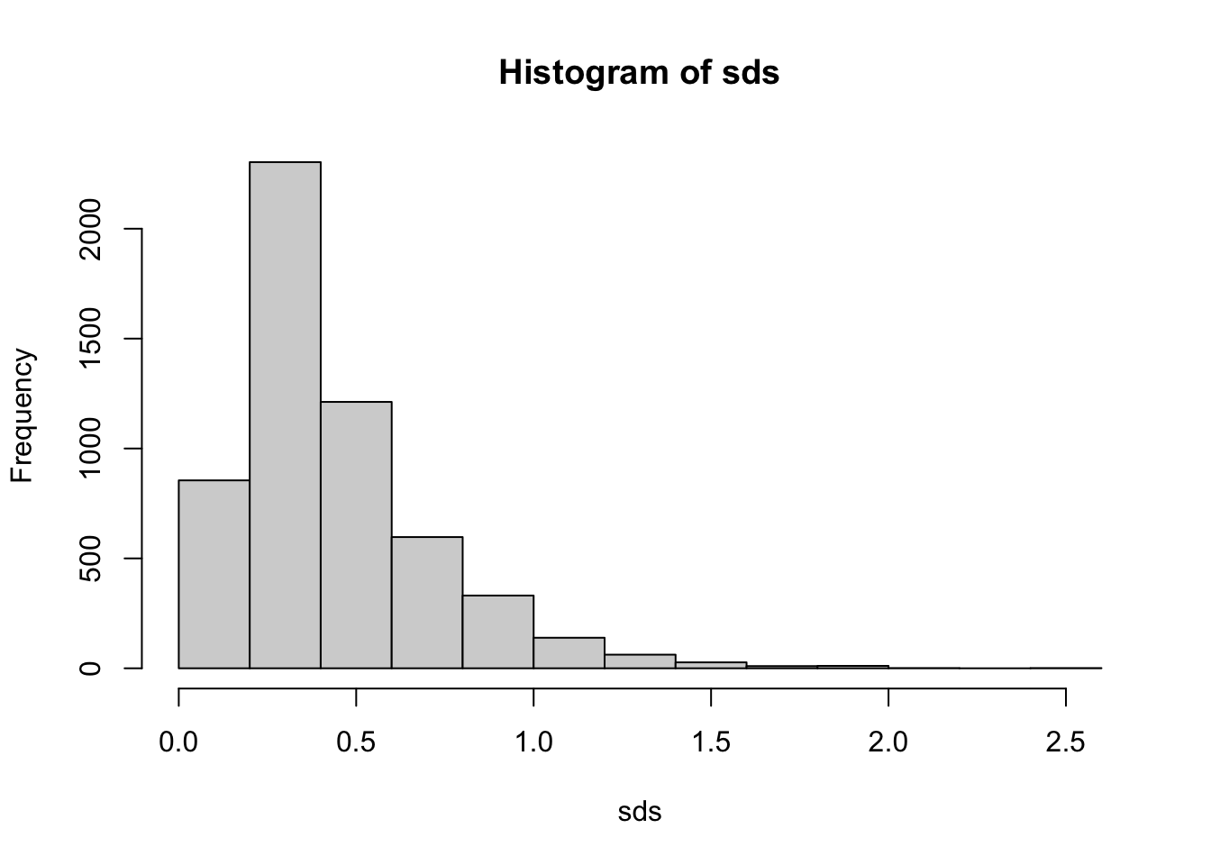
Figure 18.2 tells the story directly. The bulk of the genes pile up near zero — they hardly change across the time course and carry little information. A long tail stretches off to the right: these are the genes whose expression swings the most. A cutoff of about sd > 0.8 sits past the main pile and keeps that informative right tail. The exact value is a judgment call, which is why it’s worth re-running with a different cutoff later (one of the exercises does just that).

Now apply the cutoff (step 3) and build a smaller SummarizedExperiment holding just the highly variable genes:

idx <- sds > 0.8 & !is.na(sds)
gse_sub <- gse[idx, ]
nrow(gse_sub)

[1] 582

That trims thousands of genes down to a few hundred — a far more workable set.

18.5.4 Clustering

gse_sub now holds just the informative genes. The kmeans() function takes a matrix (rows = genes, columns = samples) and the number of clusters. Remember to seed first so the result is reproducible.

k <- 4
set.seed(42)
km <- kmeans(assays(gse_sub)[[1]], centers = k)

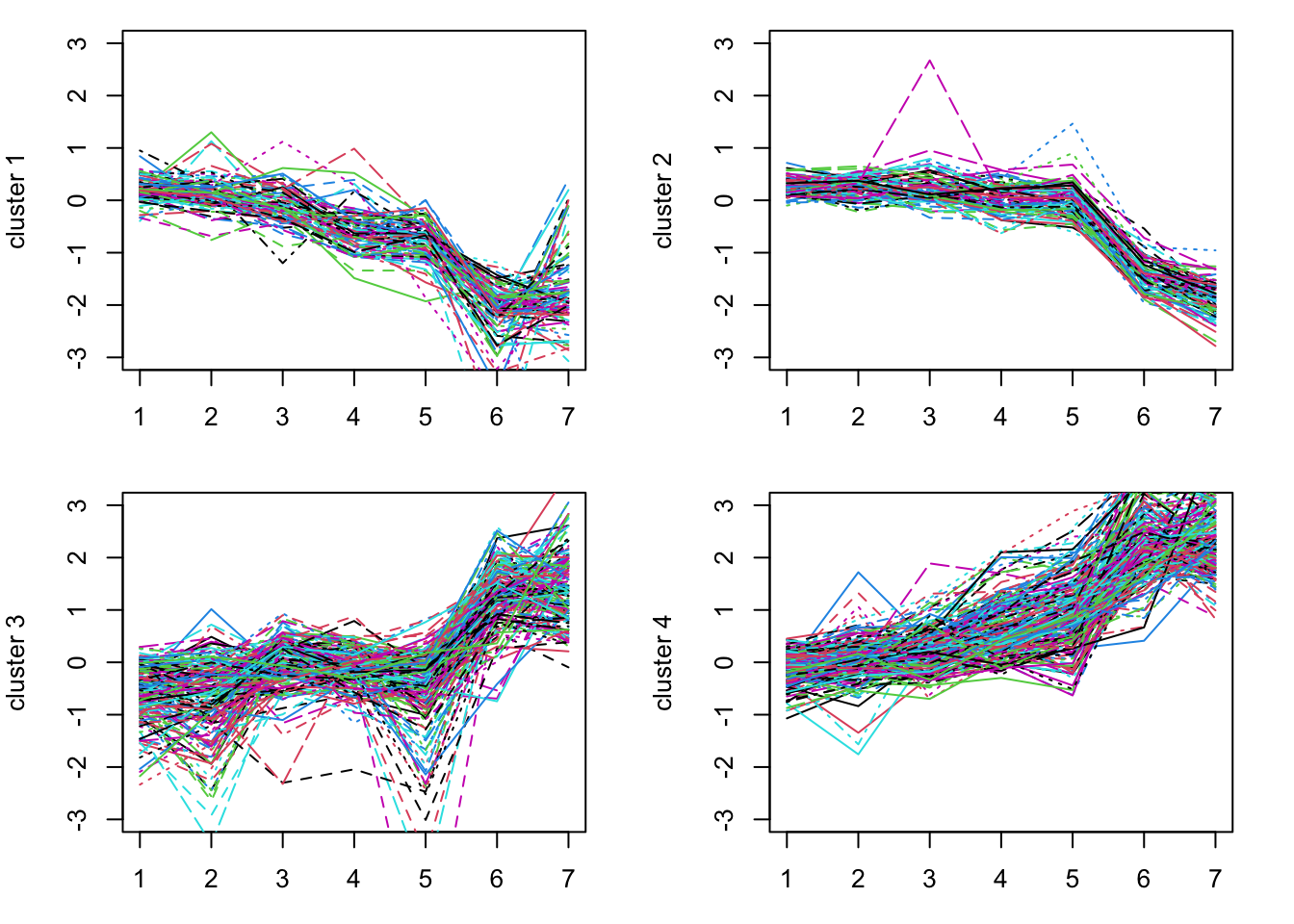
The result, km, carries a vector km$cluster that gives the cluster label (1 through k) for each gene. With four clusters, you can plot every cluster’s genes side by side and see how each group moves over time.

expression_values <- assays(gse_sub)[[1]]
par(mfrow = c(2, 2), mar = c(3, 4, 1, 2))   # 2x2 grid of plots
for (i in 1:k) {
    matplot(t(expression_values[km$cluster == i, ]), type = "l",
            ylim = c(-3, 3), ylab = paste("cluster", i))
}

Figure 18.3: Expression profiles for the four clusters found by k-means. Each line is one gene; the x-axis runs left to right across the time course, and the y-axis is the (standardized) expression level. Genes within a cluster share a trend, which suggests they may be co-regulated.

18.5.5 Reading the clusters as biology

This is the step that the numbers were building toward. Each panel in Figure 18.3 is a group of genes that move together across the time course — and “together” is the whole point, because co-regulated genes are often part of the same pathway or controlled by the same switch.

Look at the shapes rather than the exact lines:

• Some clusters rise toward the late time points. Those are genes that get switched on as the glucose runs out and the cells shift to respiration — candidate members of the respiratory and stress-response programs.
• Other clusters fall across the course. Those genes are being switched off during the shift — for example, the fermentation and growth machinery the cell no longer needs once glucose is scarce.
• The lines within each panel hug one another tightly, which is the visual signature of co-regulation: many genes responding in step to the same metabolic cue.

That is the payoff of clustering. You started with 6,400 noisy trajectories and ended with a handful of clean, interpretable patterns — rising groups, falling groups — that map directly onto the biology of the diauxic shift. If you wanted to go further, you could pull the gene names out of each cluster (rownames(gse_sub)[km$cluster == i]) and ask whether the “rising” cluster is enriched for respiration genes.

NoteWhy standardized expression?

The y-axis runs from about −3 to 3 because these microarray values are log-ratios centered near zero: positive means “higher than the reference,” negative means “lower.” Clustering on values like these groups genes by the shape of their response over time rather than by their absolute brightness, which is usually what you want.

18.6 Exercises

For each exercise, reuse the gse and gse_sub objects you built above.

1. Try a different k. Re-run the clustering with k <- 6 instead of 4 and re-make the cluster plots. Do the extra clusters reveal new patterns, or do they mostly split the existing ones?

   NoteSolution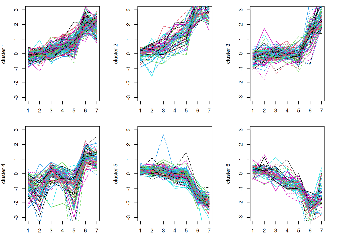

   k6 <- 6
   set.seed(42)
   km6 <- kmeans(assays(gse_sub)[[1]], centers = k6)
   par(mfrow = c(2, 3), mar = c(3, 4, 1, 2))
   for (i in 1:k6) {
       matplot(t(expression_values[km6$cluster == i, ]), type = "l",
               ylim = c(-3, 3), ylab = paste("cluster", i))
   }

   

   With more clusters, the broad “rising” and “falling” groups tend to break into finer sub-patterns (e.g. early vs. late risers). There is no single correct k; the right number depends on how fine a distinction is biologically useful.

2. Try a different cutoff. Lower the standard-deviation cutoff to 0.5 so you keep more genes, rebuild the subset, and cluster again with k = 4. How many genes do you keep now, and do the cluster shapes get cleaner or noisier?

   NoteSolution

   idx2 <- sds > 0.5 & !is.na(sds)
   gse_sub2 <- gse[idx2, ]
   nrow(gse_sub2)

   [1] 1657

   set.seed(42)
   km2 <- kmeans(assays(gse_sub2)[[1]], centers = 4)

   A lower cutoff keeps many more genes, including less-variable ones. The extra genes are noisier, so the cluster profiles usually look a little messier. This is the sensitivity check the chapter warned about: the cutoff is a knob, and it’s worth turning it to see whether your conclusions hold.

3. How big is each cluster? Using your original km result, count how many genes fall in each of the four clusters.

   NoteSolution

   table(km$cluster)

   
     1   2   3   4 
    98 102 203 179 

   table() tallies the cluster labels. Uneven cluster sizes are normal and fine — a cluster of co-regulated genes is just as real whether it has 30 members or

4. Reproducibility. Run kmeans() on gse_sub twice without calling set.seed() first, and compare table() of the cluster labels between the two runs. What changes, and why does that matter for a printed result?

   NoteSolution

   km_a <- kmeans(assays(gse_sub)[[1]], centers = 4)
   km_b <- kmeans(assays(gse_sub)[[1]], centers = 4)
   table(km_a$cluster)

   
     1   2   3   4 
    91  88 165 238 

   table(km_b$cluster)

   
     1   2   3   4 
   165  91  88 238 

   The two runs start from different random centroids, so the cluster labels (and sometimes the exact membership) differ. Seeding with set.seed() pins the random start so anyone re-running your code sees the same clusters — which is exactly why we seeded the worked example.

18.7 Summary

You set out to find groups of genes that behave alike across the yeast diauxic shift, and you did it with k-means. Looking back at the objectives:

• You can describe k-means as an unsupervised method that sorts points into k groups around moving centroids, and you know its main trade-offs (you pick k; it likes round, even clusters; it’s sensitive to outliers and to the random start).
• You pulled a real dataset from GEO with getGEO() and converted it to a SummarizedExperiment.
• You filtered the genes down to the high-variance, informative ones using their standard deviation, and you saw on Figure 18.2 why a cutoff past the main pile makes sense.
• You ran kmeans() reproducibly with set.seed() and plotted each cluster.
• You read Figure 18.3 as biology: clusters that rise are genes switched on for respiration as glucose runs out, and clusters that fall are the fermentation/growth machinery being switched off — co-regulated genes moving in step through the diauxic shift.

That wraps up the statistics part of the book. Clustering is your first taste of unsupervised learning; the machine-learning chapters pick up that thread and build on it.

Bourgon, Richard, Robert Gentleman, and Wolfgang Huber. 2010. “Independent Filtering Increases Detection Power for High-Throughput Experiments.” Proceedings of the National Academy of Sciences 107 (21): 9546–51. https://doi.org/10.1073/pnas.0914005107.

DeRisi, J. L., V. R. Iyer, and P. O. Brown. 1997. “Exploring the Metabolic and Genetic Control of Gene Expression on a Genomic Scale.” Science (New York, N.Y.) 278 (5338): 680–86. https://doi.org/10.1126/science.278.5338.680.