22 The t-statistic and t-distribution

Author

Affiliation

University of Colorado
Anschutz School of Medicine

Published

June 1, 2024

Modified

June 11, 2026

Suppose you measure a gene’s expression in five treated samples and five controls, and the treated mean comes out higher. Is that a real effect, or just the kind of gap you’d expect by chance from five noisy measurements? With only a handful of samples you can’t lean on the normal distribution as-is, because you had to estimate the variability from the same tiny sample you’re testing. The t-distribution is the honest accounting for that extra uncertainty — and in this chapter we’ll build it by simulation so you can see exactly where it comes from, then use R’s t.test() to put it to work.

The distribution that the t-statistic follows was described in a famous 1908 paper (Student 1908) by “Student” — a pseudonym for William Sealy Gosset, who worked at the Guinness brewery and published anonymously because his employer treated statistical methods as a trade secret.

22.1 What you’ll learn

Explain why estimating the standard deviation from a small sample forces us off the normal distribution and onto the t-distribution.
Read a Z-score and a t-score and say what each one measures.
Use simulation to show that t-based p-values are calibrated (uniform under the null hypothesis) when the normal-based ones are not.
Run one-sample, two-sample, and formula-based tests with t.test().
Estimate statistical power with power.t.test() and by simulation.

22.2 Background

A t-test is a statistical hypothesis test you reach for when you want to compare means and you only have a sample to work from. It comes in three everyday flavors:

One-sample — compare a sample mean to a single hypothesized or target value.
Two-sample — compare the means of two groups.
Paired — compare two measurements on the same units (e.g., before-and-after on the same patients).

A t-test combines three ingredients — the t-statistic, the t-distribution, and the degrees of freedom — to decide whether a difference is bigger than chance would comfortably produce. (To compare three or more means at once you’d reach instead for an analysis of variance, or ANOVA.)

We’ll get to t.test(), but the point of this chapter is to first see why the t-distribution exists. That story starts with something you may already have met: the Z-score.

22.3 The Z-score and probability

Before we talk about t-scores, let’s review the Z-score, its relationship to the normal distribution, and how it turns into a probability.

The Z-score is defined as:

\[Z = \frac{x - \mu}{\sigma} \tag{22.1}\]

where $\mu$ is the population mean that $x$ is drawn from and $\sigma$ is the population standard deviation — taken as known, not estimated from the data. In words: a Z-score says how many standard deviations a value sits from the mean.

The probability of observing a Z-score of $z$ or smaller can be calculated with pnorm(z, mu, sigma).

For example, suppose our “population” is known and truly has a mean of 0 and a standard deviation of 1 (the standard normal). For any observation drawn from that population, we can assign a probability of seeing a value that extreme by random chance — under the assumption that the null hypothesis is TRUE.

zscore <- seq(-5, 5, 1)

For each value of zscore, let’s calculate the probability and collect the results in a data.frame. We’ll name it pdat (for “probability data”) so it doesn’t collide with the df we use later for degrees of freedom.

pdat <- data.frame(
    zscore = zscore,
    pval   = pnorm(zscore, 0, 1)
)
pdat

   zscore         pval
1      -5 2.866516e-07
2      -4 3.167124e-05
3      -3 1.349898e-03
4      -2 2.275013e-02
5      -1 1.586553e-01
6       0 5.000000e-01
7       1 8.413447e-01
8       2 9.772499e-01
9       3 9.986501e-01
10      4 9.999683e-01
11      5 9.999997e-01

Why is the p-value for something 5 standard deviations above the mean (zscore = 5) nearly 1 here? Because pnorm reports the lower tail by default — the probability of a value at or below z. A value 5 standard deviations above the mean has almost the entire distribution below it, so that probability is nearly 1.

Let’s plot probability against Z-score:

plot(pdat$zscore, pdat$pval, type = 'b')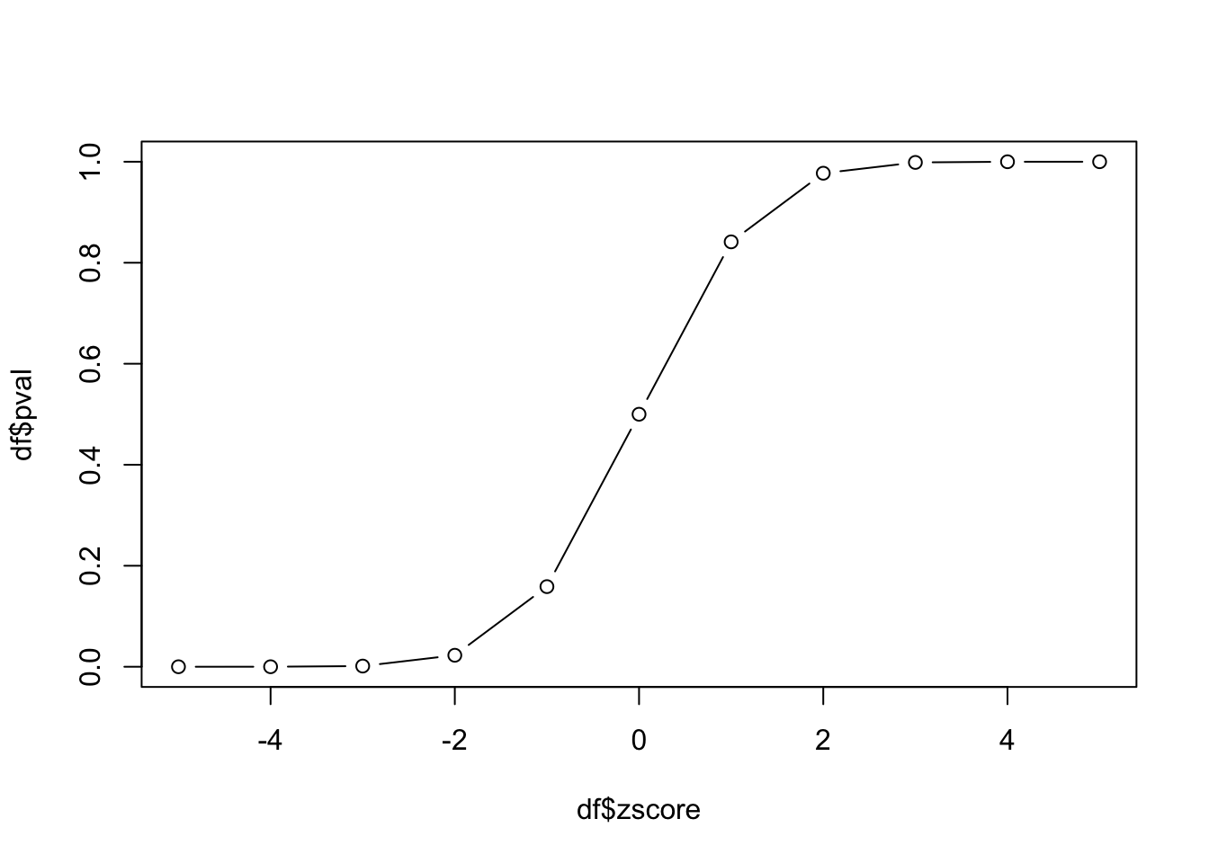

This curve is the cumulative distribution function (CDF). Read it like a lookup table: pick a Z-score on the x-axis and read off the probability of seeing a value that small. Because we built our example to follow the standard normal, this is also the CDF of the standard normal distribution.

What a p-value is (and isn’t)

A p-value is the probability of a result at least this extreme if the null hypothesis were true. It is not the probability that the null hypothesis is true, and a small p-value is not a measure of effect size. For an accessible, authoritative take on the common misreadings, see the American Statistical Association’s statement on p-values (Wasserstein and Lazar 2016).

22.3.1 Small diversion: a two-sided pnorm

pnorm returns a one-sided probability using the lower tail by default. Often we don’t care which direction a value deviates — only that it’s far from the mean — so we want a two-sided p-value. We can build one in three steps:

Take the absolute value of x, so direction no longer matters.
Call pnorm with lower.tail = FALSE, so larger |x| gives smaller probabilities.
Multiply by 2 to count both tails.

twosidedpnorm <- function(x, mu = 0, sd = 1) {
    2 * pnorm(abs(x), mu, sd, lower.tail = FALSE)
}

Now we can ask how surprising it is to land 2 or 3 standard deviations from the mean in either direction:

twosidedpnorm(2)

[1] 0.04550026

twosidedpnorm(3)

[1] 0.002699796

22.4 The t-distribution

Everything above leaned on one big assumption: that we know the standard deviation $\sigma$. Recall the Z-score:

\[Z = \frac{x - \mu}{\sigma}\]

and the population standard deviation:

\[\sigma = \sqrt{\frac{1}{N}\sum_{i=1}^{N}(x_i - \mu)^2} \tag{22.2}\]

When we genuinely know $\sigma$, the Z-score is the right tool. But usually we only have a sample, not the whole population. Then we swap the Z-score for the t-score:

\[t = \frac{x - \bar{x}}{s} \tag{22.3}\]

This looks almost identical to the Z-score, with two changes: we use the sample mean $\bar{x}$ in place of $\mu$, and we estimate the standard deviation as $s$ from the data:

\[s = \sqrt{\frac{1}{N-1}\sum_{i=1}^{N}(x_i - \bar{x})^2} \tag{22.4}\]

In words: the sample standard deviation $s$ is the typical distance of a data point from the sample mean. The only change from the population formula is the divisor — $N-1$ instead of $N$ — which corrects for the fact that we used the data twice: once to estimate the mean, and again to measure the spread around it.

The whole point of the t-distribution

Because we estimate the standard deviation from a small sample, our test statistic is more uncertain than a Z-score. The t-distribution captures that by having fatter tails for small samples — so it takes a more extreme result to reach significance. As the sample grows, the estimate sharpens and the t-distribution slides back toward the normal.

We can see those fatter tails. Let’s plot the t-distribution densities for 3, 6, 10, and 20 degrees of freedom (smaller degrees of freedom means a smaller sample) alongside the normal:

library(dplyr)
library(ggplot2)
t_values <- seq(-6, 6, 0.01)
tdens <- data.frame(
    value  = t_values,
    t_3    = dt(t_values, 3),
    t_6    = dt(t_values, 6),
    t_10   = dt(t_values, 10),
    t_20   = dt(t_values, 20),
    Normal = dnorm(t_values)
) |>
    tidyr::pivot_longer(-value, names_to = "Distribution", values_to = "density")
ggplot(tdens, aes(x = value, y = density, color = Distribution)) +
    geom_line()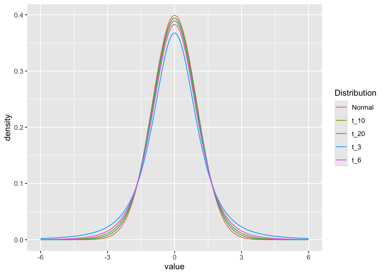

Figure 22.1: t-distributions for various degrees of freedom. The tails are fatter for smaller degrees of freedom — the visible cost of estimating the standard deviation from the data.

The dt and dnorm functions give the density (the height of the curve) at each point. Notice how the t_3 curve sits lowest in the middle and highest in the tails — that extra tail weight is the uncertainty from a tiny sample, drawn to scale.

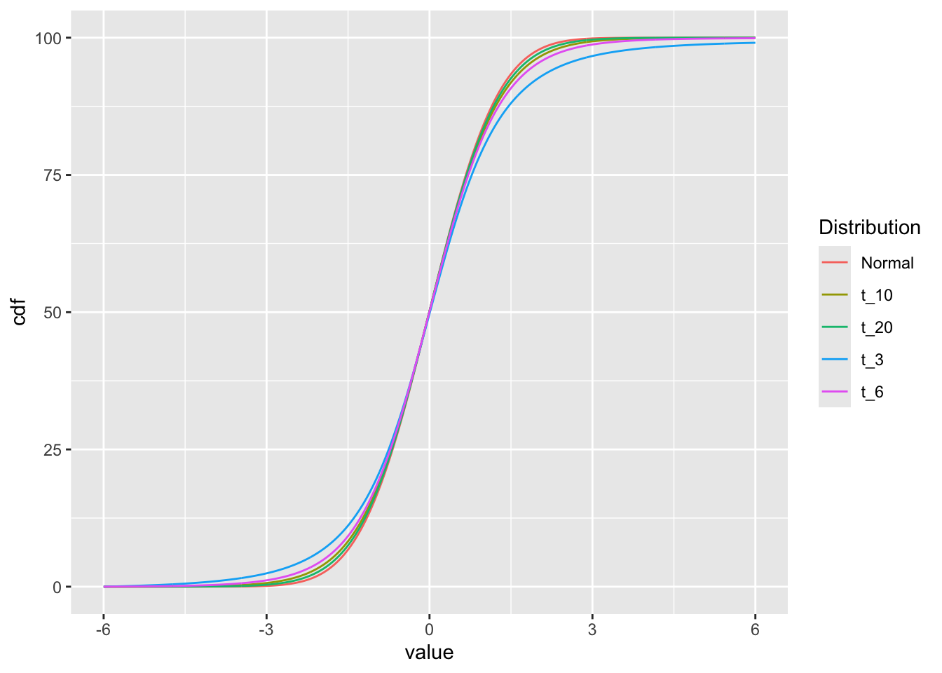
We can also look at the cumulative version of each curve:

tcdf <- tdens |>
    group_by(Distribution) |>
    arrange(value) |>
    mutate(cdf = cumsum(density))
ggplot(tcdf, aes(x = value, y = cdf, color = Distribution)) +
    geom_line()

22.4.1 p-values based on Z vs t

When we have a sample and want to test how far its mean sits from a population mean, we scale by the standard error (the standard deviation of the sample mean), $\sigma/\sqrt{n}$:

\[z = \frac{x - \mu}{\sigma/\sqrt{n}}\]

Let’s compare the p-value we’d get from the normal distribution against the one from the t-distribution, for a single small sample.

set.seed(5432)
samp <- rnorm(5, mean = 0.5)
z <- sqrt(length(samp)) * mean(samp)  # simplifying assumption: sigma = 1, mu = 0

The p-value if we pretend we know the standard deviation:

pnorm(z, lower.tail = FALSE)

[1] 0.02428316

In reality we don’t know it, so we estimate it from the data with sd() and use the t-distribution (with length(samp) - 1 degrees of freedom):

ts <- sqrt(length(samp)) * mean(samp) / sd(samp)
pnorm(ts, lower.tail = FALSE)                      # wrong: treats the estimate as known

[1] 0.0167297

pt(ts, df = length(samp) - 1, lower.tail = FALSE)  # right: accounts for the estimate

[1] 0.0503001

The two numbers differ, and that difference is the whole story: using the normal distribution on an estimated standard deviation quietly understates our uncertainty. The next section makes that mistake visible at scale.

22.4.2 Experiment: does the choice of distribution actually matter?

Here’s a claim worth testing for yourself rather than taking on faith: if you estimate the standard deviation but compute p-values from the normal distribution, your p-values will be wrong. Let’s find out how wrong.

There’s a tidy way to check. If a test is working correctly, then under the null hypothesis its p-values should be uniformly distributed between 0 and 1 — every value equally likely. So we’ll simulate many samples where the null is true, compute p-values three ways, and look at the histograms. A flat histogram means the test is honest; a lopsided one means it isn’t.

The plan:

Draw many samples of size n from the standard normal distribution.
Score each with the Z-statistic (pretending we know $\sigma$).
Score each with the t-statistic (estimating $\sigma$ from the data), then compute p-values two ways — from the normal, and from the t-distribution.

First, a function that draws a sample and returns its Z-score:

zf <- function(n) {
    samp <- rnorm(n)
    sqrt(length(samp)) * mean(samp) / 1  # simplifying assumption: sigma = 1, mu = 0
}

Give it a try:

zf(5)

[1] 0.7406094

Run 10,000 replicates and look at the p-value histogram. Here we do know the population standard deviation (we’re sampling from the standard normal), so the normal distribution is the correct choice — and the histogram should be flat:

z10k <- replicate(10000, zf(5))
hist(pnorm(z10k))

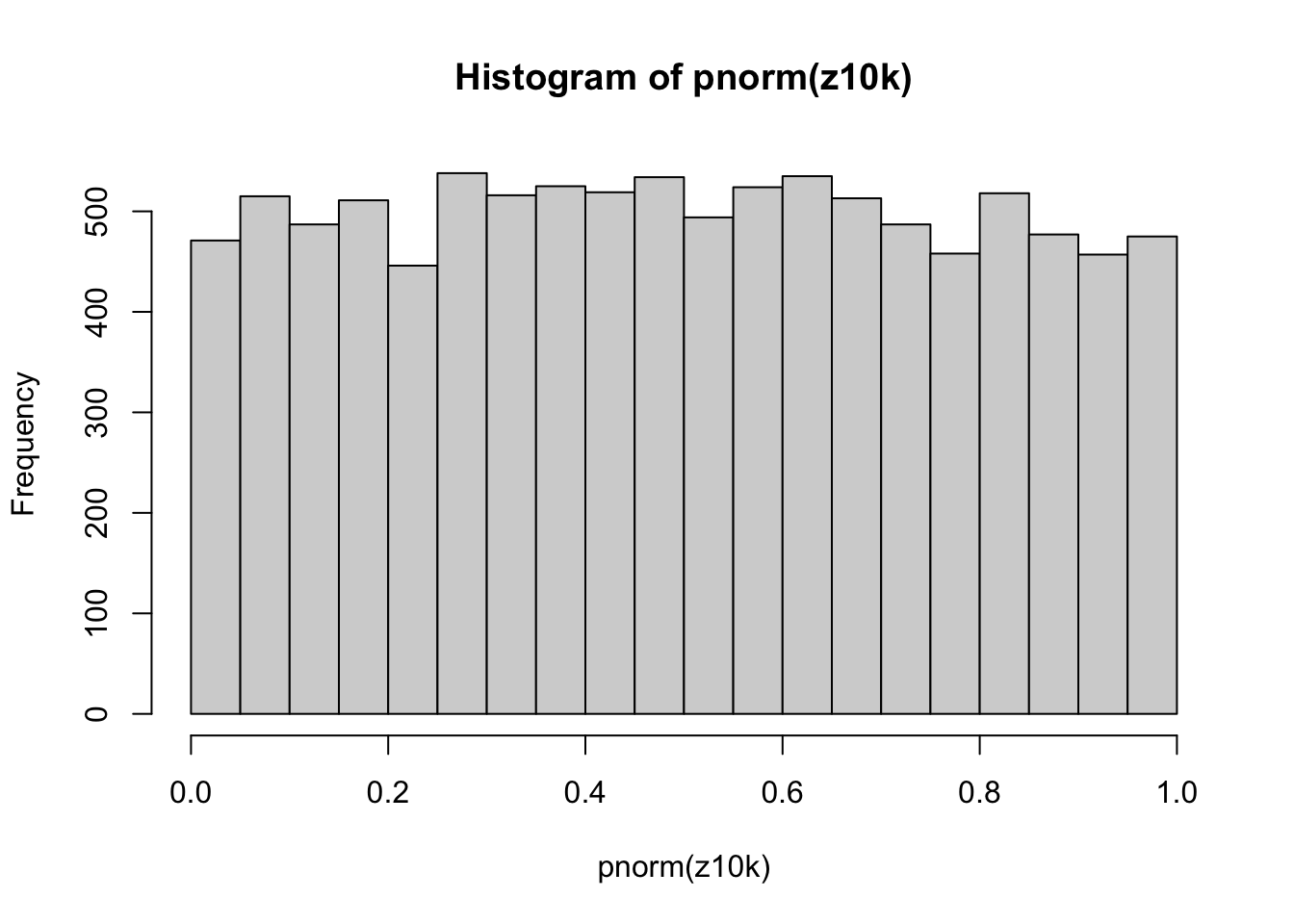
Flat, as promised. Now the t-score function — same idea, but we estimate the standard deviation with sd() instead of assuming it:

tf <- function(n) {
    samp <- rnorm(n)
    # use the sample standard deviation, since we "don't know" the population one
    sqrt(length(samp)) * mean(samp) / sd(samp)
}

If we feed those t-scores to the normal distribution — the common mistake — the histogram is no longer flat:

t10k <- replicate(10000, tf(5))
hist(pnorm(t10k))

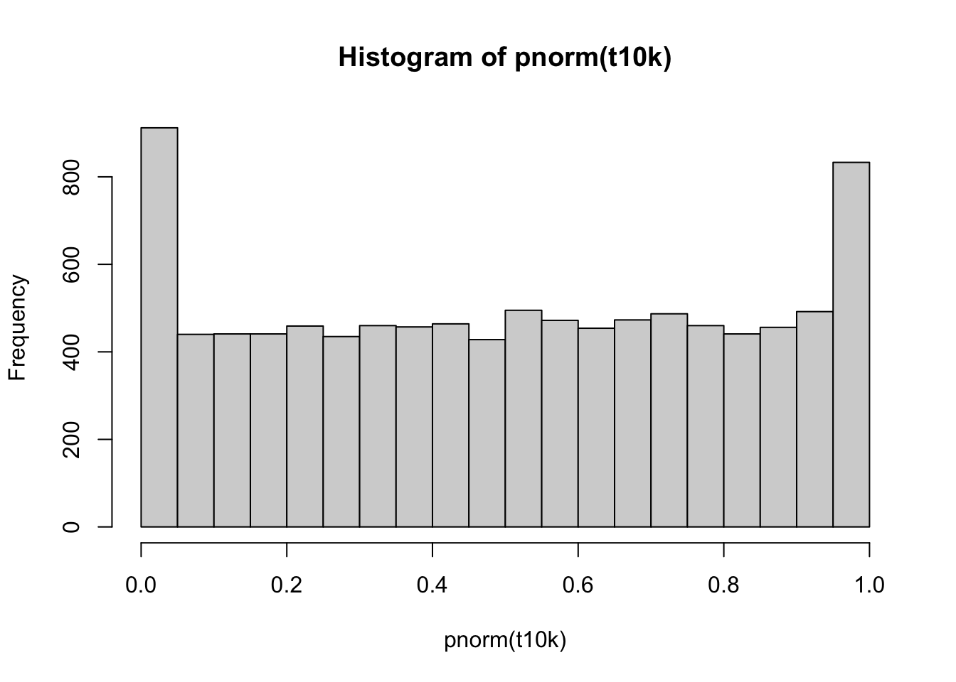
The pile-ups near 0 and 1 mean this test rejects the null too often: it’s overconfident, exactly because it treats an estimated standard deviation as if it were known. Now feed the same t-scores to the t-distribution (with n - 1 = 4 degrees of freedom):

hist(pt(t10k, 4))

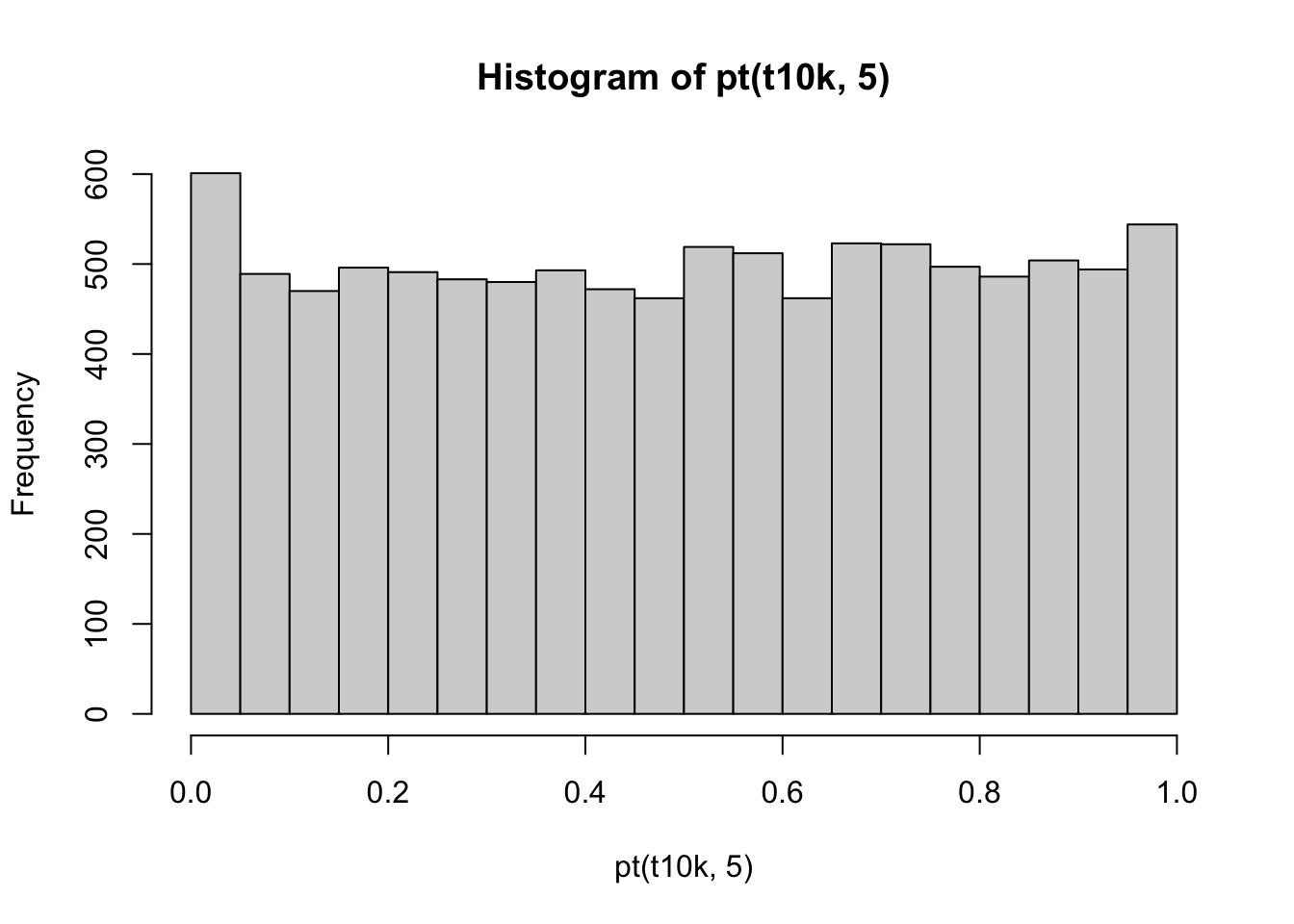
Flat again. The t-distribution restores honest, uniform p-values — that is the payoff for all the math above.

We can also compare the two sets of scores directly with a Q-Q plot.

A Q-Q plot plots the quantiles of two distributions against each other. If the two distributions are identical, the points fall on a straight line; where they differ, the points peel away from it.

Here we compare our simulated z-scores against our simulated t-scores. Because the t-scores carry the extra uncertainty from estimating the standard deviation, we expect them to disagree with the z-scores in the tails.

qqplot(z10k, t10k)
abline(0, 1)

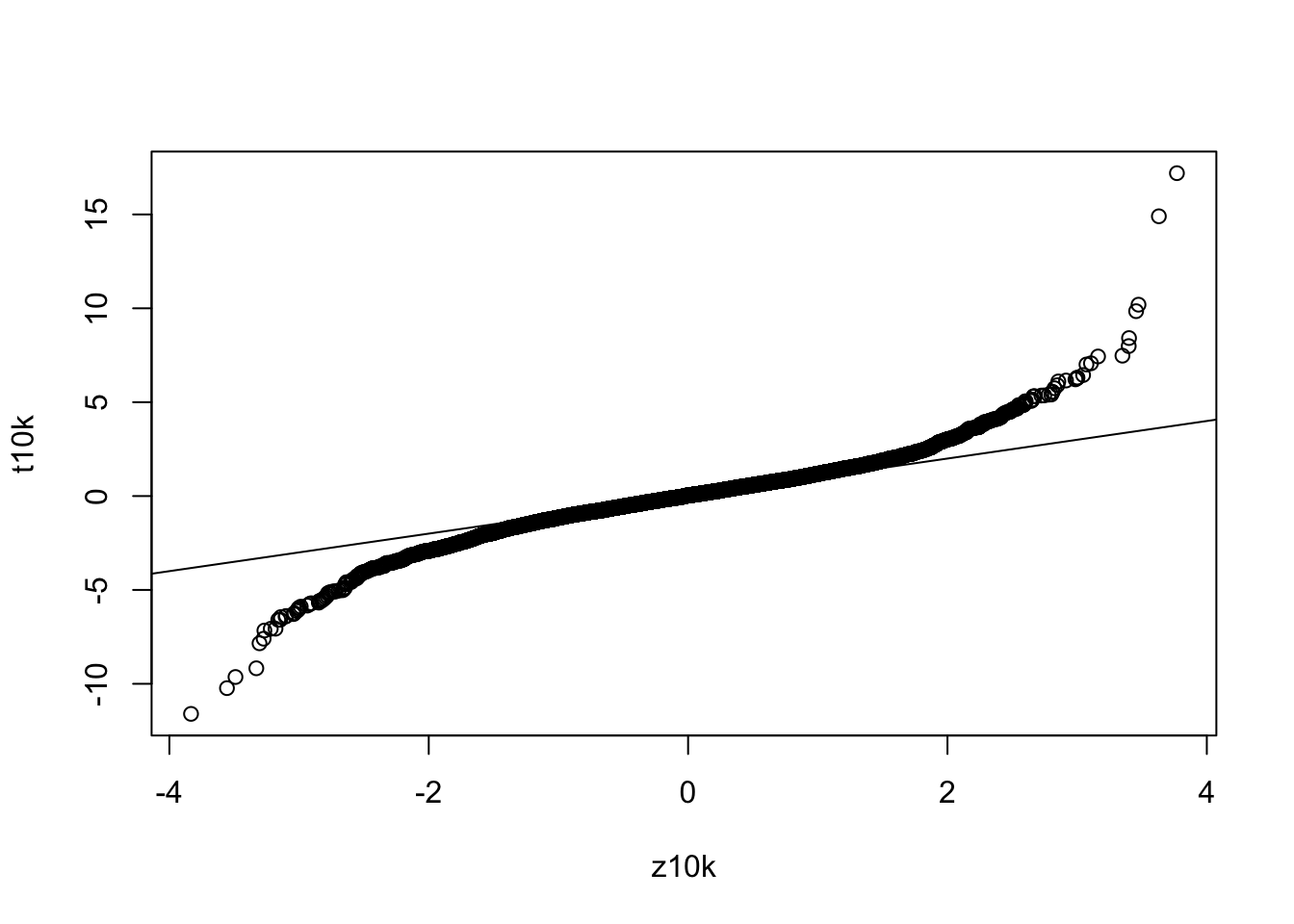
The points bow away from the line at both ends — the t-distribution’s fatter tails, made visible. What would happen if you raised the sample size from 5 to 50? Try it: the bow should shrink as the t-distribution approaches the normal.

22.5 Checkpoint: t vs normal

Before we start using t.test(), let’s pin down the one idea this chapter has been circling.

The t-distribution is a family of distributions indexed by the degrees of freedom, which track the sample size. It has heavier tails than the normal for small samples and approaches the normal as the sample grows. Those heavier tails make it more conservative — it takes a more extreme result to reach significance — which is the correct response to the uncertainty introduced by estimating the standard deviation from the data. That correction matters most exactly when you have the least data.

22.6 t.test

Now the practical part. R’s t.test() packages everything above into one function — you hand it data, it returns a t-statistic, degrees of freedom, a p-value, and a confidence interval.

22.6.1 One-sample

A one-sample test compares a sample mean to a single value (zero, by default). We’ll simulate a sample whose true mean is 1, so we know the answer the test should be reaching for.

x <- rnorm(20, 1)
# small sample: just the first 5 values
t.test(x[1:5])


    One Sample t-test

data:  x[1:5]
t = 0.97599, df = 4, p-value = 0.3843
alternative hypothesis: true mean is not equal to 0
95 percent confidence interval:
 -1.029600  2.145843
sample estimates:
mean of x 
0.5581214

We rigged this so the null hypothesis (mean = 0) is false — the true mean is 1. But with only 5 values the evidence is thin, so the p-value is modest. Add more data and the effect comes through clearly:

t.test(x[1:20])


    One Sample t-test

data:  x[1:20]
t = 3.8245, df = 19, p-value = 0.001144
alternative hypothesis: true mean is not equal to 0
95 percent confidence interval:
 0.3541055 1.2101894
sample estimates:
mean of x 
0.7821474

22.6.2 Two-sample

A two-sample test compares the means of two groups:

x <- rnorm(10, 0.5)
y <- rnorm(10, -0.5)
t.test(x, y)


    Welch Two Sample t-test

data:  x and y
t = 3.4296, df = 17.926, p-value = 0.003003
alternative hypothesis: true difference in means is not equal to 0
95 percent confidence interval:
 0.5811367 2.4204048
sample estimates:
 mean of x  mean of y 
 0.7039205 -0.7968502

22.6.3 From a data frame

Often your data and group labels live in two columns of a data frame rather than in two separate vectors:

tdat <- data.frame(
    value = c(x, y),
    group = as.factor(rep(c('g1', 'g2'), each = 10))
)
tdat

         value group
1   1.12896674    g1
2  -1.26838101    g1
3   1.04577597    g1
4   1.69075585    g1
5   0.18672204    g1
6   1.99715092    g1
7   1.15424947    g1
8   0.37671442    g1
9  -0.09565723    g1
10  0.82290783    g1
11 -1.48530261    g2
12 -1.29200440    g2
13 -0.18778362    g2
14  0.59205742    g2
15 -2.10065248    g2
16 -0.29961560    g2
17 -0.38985115    g2
18 -2.47126235    g2
19 -0.63654380    g2
20  0.30245611    g2

R lets you run the same test with formula notation:

t.test(value ~ group, data = tdat)


    Welch Two Sample t-test

data:  value by group
t = 3.4296, df = 17.926, p-value = 0.003003
alternative hypothesis: true difference in means between group g1 and group g2 is not equal to 0
95 percent confidence interval:
 0.5811367 2.4204048
sample estimates:
mean in group g1 mean in group g2 
       0.7039205       -0.7968502

Read value ~ group as “value is a function of group” — in practice, do a t-test of the values in g1 against those in g2.

22.6.4 Equivalence to a linear model

A two-sample t-test (with equal variances assumed) is really a linear model in disguise. Run the test:

t.test(value ~ group, data = tdat, var.equal = TRUE)


    Two Sample t-test

data:  value by group
t = 3.4296, df = 18, p-value = 0.002989
alternative hypothesis: true difference in means between group g1 and group g2 is not equal to 0
95 percent confidence interval:
 0.5814078 2.4201337
sample estimates:
mean in group g1 mean in group g2 
       0.7039205       -0.7968502

and compare it to fitting a line:

res <- lm(value ~ group, data = tdat)
summary(res)


Call:
lm(formula = value ~ group, data = tdat)

Residuals:
    Min      1Q  Median      3Q     Max 
-1.9723 -0.5600  0.2511  0.5252  1.3889 

Coefficients:
            Estimate Std. Error t value Pr(>|t|)   
(Intercept)   0.7039     0.3094   2.275  0.03538 * 
groupg2      -1.5008     0.4376  -3.430  0.00299 **
---
Signif. codes:  0 '***' 0.001 '**' 0.01 '*' 0.05 '.' 0.1 ' ' 1

Residual standard error: 0.9785 on 18 degrees of freedom
Multiple R-squared:  0.3952,    Adjusted R-squared:  0.3616 
F-statistic: 11.76 on 1 and 18 DF,  p-value: 0.002989

The groupg2 coefficient is the difference in means, and its p-value matches the t-test’s. Same question, same answer, two front doors.

22.7 Power calculations

The power of a test is the probability that it correctly rejects the null hypothesis when the alternative is true — in other words, the probability of not missing a real effect (not making a Type II error). Power rises with the significance level (alpha), the sample size, and the effect size. It’s what you compute before an experiment to ask “how many samples do I need?”

power.t.test() ties these quantities together. From help("power.t.test"), the main arguments are:

n — sample size
delta — effect size (difference in means)
sd — standard deviation
sig.level — significance level
power — power

You supply any four and it solves for the fifth. For example, the power of a one-sample test with n = 5, sd = 1, and an effect size of 1:

power.t.test(n = 5, delta = 1, sd = 1, sig.level = 0.05)


     Two-sample t test power calculation 

              n = 5
          delta = 1
             sd = 1
      sig.level = 0.05
          power = 0.2859276
    alternative = two.sided

NOTE: n is number in *each* group

That prints a full summary. To grab just the power value, use $:

power.t.test(n = 5, delta = 1, sd = 1,
             sig.level = 0.05, type = 'one.sample')$power

[1] 0.4013203

Tip

When a function returns a result that doesn’t look “computable” — like the summary from power.t.test — you can pull out a single piece with $. How do you know what’s available to extract? Use names() for the labels, or str() for the full structure:

names(power.t.test(n = 5, delta = 1, sd = 1,
             sig.level = 0.05, type = 'one.sample'))

[1] "n"           "delta"       "sd"          "sig.level"   "power"      
[6] "alternative" "note"        "method"

# or
str(power.t.test(n = 5, delta = 1, sd = 1,
             sig.level = 0.05, type = 'one.sample'))

List of 8
 $ n          : num 5
 $ delta      : num 1
 $ sd         : num 1
 $ sig.level  : num 0.05
 $ power      : num 0.401
 $ alternative: chr "two.sided"
 $ note       : NULL
 $ method     : chr "One-sample t test power calculation"
 - attr(*, "class")= chr "power.htest"

Just as often you’ll flip the question around: how big a sample do I need to hit a target power? Solve for n by supplying power instead:

power.t.test(delta = 1, sd = 1, sig.level = 0.05, power = 0.8, type = "one.sample")


     One-sample t test power calculation 

              n = 9.937864
          delta = 1
             sd = 1
      sig.level = 0.05
          power = 0.8
    alternative = two.sided

power.t.test is convenient and fast. But as we saw with the t-distribution itself, sometimes the distribution of a test statistic is not easily calculated in closed form. In those cases we can estimate power by simulation — run the experiment thousands of times and count how often it rejects the null:

sim_t_test_pval <- function(n = 5, delta = 1, sd = 1, sig.level = 0.05) {
    x <- rnorm(n, delta, sd)
    t.test(x)$p.value <= sig.level
}
pow <- mean(replicate(1000, sim_t_test_pval()))
pow

[1] 0.405

Step by step: sim_t_test_pval simulates one sample of size n from a normal distribution with mean delta and standard deviation sd, runs a one-sample t-test, and returns TRUE when the p-value clears the significance threshold. replicate repeats that 1000 times, and mean turns the resulting TRUE/FALSE vector into the proportion of significant results — our estimate of power.

The two approaches should land in the same place:

power.t.test(n = 5, delta = 1, sd = 1, sig.level = 0.05, type = 'one.sample')$power

[1] 0.4013203

mean(replicate(1000, sim_t_test_pval(n = 5, delta = 1, sd = 1, sig.level = 0.05)))

[1] 0.414

Close — and the simulation route keeps working in situations where no neat formula exists.

22.8 Exercises

Note

Several exercises reuse objects (samp, t10k, tdat) built earlier in the chapter. Run the chapter’s chunks first, or recreate the objects in your session.

One-sided vs two-sided. Use twosidedpnorm() to find the two-sided p-value for a Z-score of 1.96. Does the answer match the “95%” rule of thumb you may have heard?
NoteSolution
twosidedpnorm(1.96)

[1] 0.04999579
It’s almost exactly 0.05 — which is why 1.96 is the classic cutoff for a two-sided test at the 5% level.
Degrees of freedom matter. Compute the two-sided p-value for t = 2.5 from the t-distribution with 4 degrees of freedom and again with 30. Which is larger, and does that fit the “fatter tails” story?
NoteSolution
2 * pt(2.5, df = 4, lower.tail = FALSE)

[1] 0.06676654

2 * pt(2.5, df = 30, lower.tail = FALSE)

[1] 0.01811565
The 4-df p-value is larger. Fewer degrees of freedom means fatter tails, so the same t-statistic is less surprising — it takes more extreme evidence to reach significance with a small sample.

A paired test. Imagine the same 8 patients measured before and after a treatment. Simulate the pairs below and run a paired t-test with t.test(after, before, paired = TRUE). How does the result compare to treating the two groups as independent (paired = FALSE)?

set.seed(11)
before <- rnorm(8, 10, 2)
after  <- before + rnorm(8, 1, 0.5)  # a real, consistent bump per patient

Solution

t.test(after, before, paired = TRUE)


 Paired t-test

data:  after and before
t = 6.7665, df = 7, p-value = 0.0002611
alternative hypothesis: true mean difference is not equal to 0
95 percent confidence interval:
 0.4408169 0.9144199
sample estimates:
mean difference 
      0.6776184

t.test(after, before, paired = FALSE)


 Welch Two Sample t-test

data:  after and before
t = 0.62439, df = 13.955, p-value = 0.5424
alternative hypothesis: true difference in means is not equal to 0
95 percent confidence interval:
 -1.650735  3.005972
sample estimates:
mean of x mean of y 
10.364923  9.687305

The paired test has a much smaller p-value. By matching each patient to themselves it removes the patient-to-patient variability, leaving only the change due to treatment — so it detects the effect that the unpaired test can barely see.

Power and sample size. Using power.t.test, find the sample size needed to detect an effect of delta = 0.5 (with sd = 1) at 80% power for a one-sample test. Then halve the effect size to 0.25 and recompute. Roughly how does the required n change?
NoteSolution
power.t.test(delta = 0.5, sd = 1, sig.level = 0.05, power = 0.8, type = "one.sample")$n

[1] 33.3672

power.t.test(delta = 0.25, sd = 1, sig.level = 0.05, power = 0.8, type = "one.sample")$n

[1] 127.5161
Halving the effect size roughly quadruples the required sample size — small effects are expensive to detect. This is the single most useful intuition to carry out of a power calculation.

22.9 Summary

You can now:

Explain why estimating the standard deviation from a small sample pushes us from the normal distribution onto the t-distribution, and what “fatter tails” buys you.
Distinguish a Z-score from a t-score and turn either into a p-value with pnorm and pt.
Use simulation to check that a test is honest — uniform p-values under the null — rather than taking it on trust.
Run one-sample, two-sample, paired, and formula-based tests with t.test(), and recognize the two-sample t-test as a linear model.
Estimate power and required sample size with power.t.test() and by simulation.

The thread tying it all together: when you estimate uncertainty from your data instead of knowing it, you have to pay for that estimate — and the t-distribution is how statistics keeps the books honest.

22.10 Resources

The pwr package for a fuller toolkit of power calculations.
The American Statistical Association’s statement on p-values (Wasserstein and Lazar 2016) for what a p-value does and doesn’t tell you.