9 A primer on biological assays
Somewhere in this book you will be handed a spreadsheet with 20,000 rows and 100 columns and told to find the rows that matter. You will run the statistics, draw the figure, and reach a conclusion — all without ever touching a test tube. But to trust that conclusion you need to know what the numbers in that spreadsheet actually are. Where did a row come from? What does a single number in the table physically represent? Why is one experiment a tidy matrix of counts and another a ragged list of positions on a chromosome?
This chapter answers those questions. It is the one chapter in the book with no R code at all — it is here to give readers from a non-biological background the mental picture that the rest of the book quietly assumes. We will start with the smallest amount of cell biology you need (just enough to make the data make sense), then walk through the six experimental techniques — the assays — that produce nearly every dataset you will meet later. For each one, the goal is the same: what biological question does it answer, and what shape does its data take?
If you already know a promoter from an enhancer, skim this and move on. If you don’t, read it once and the later chapters will stop feeling like they’re written in code.
9.1 What you’ll learn
By the end of this chapter you will be able to:
- Explain, in plain language, what a gene is and what the central dogma describes.
- Describe the single idea — counting molecules — that unites most modern assays.
- For each of the six assays used in this book, state the biological question it answers and the shape of data it produces.
- Recognize which chapter later in the book works with each kind of data, so you know where each assay reappears.
- Read a figure or a methods section and place the experiment into one of these six families.
This is a primer. Every section here is a deliberate simplification of a field that people spend careers on. The aim is a working mental model, not completeness. Where a detail matters for the analysis you’ll do later, the relevant chapter fills it in.
9.2 The cell, the genome, and the central dogma
Every cell in your body carries the same instruction manual: a long molecule of DNA, packaged into chromosomes and collectively called the genome. The human genome is about three billion letters long, written in a four-letter alphabet (A, C, G, T). A gene is a stretch of that sequence that spells out a specific product — most often a protein, the molecular machines and building blocks that actually do the work of a cell.
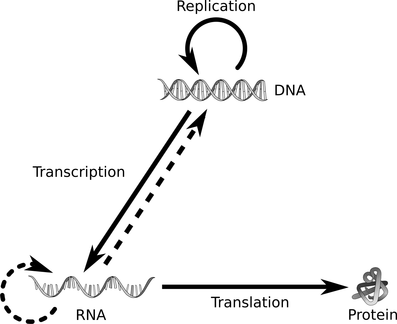
The flow of information from DNA to a working product is so central that it has a name: the central dogma of molecular biology (Figure 9.1). DNA is transcribed into a temporary working copy called RNA; a particular kind of RNA, messenger RNA (mRNA), is then translated into protein. A useful analogy: the genome is a reference library that never leaves the building; RNA is the photocopy a worker carries to the bench; protein is the thing they build from it.
Here is the fact that makes the whole book possible: every cell has the same genome, but not every gene is switched on in every cell. A neuron and a liver cell carry identical DNA, yet they look and behave completely differently because they express different genes — they transcribe different stretches of DNA into RNA, in different amounts. A gene that is “on” is being transcribed into many RNA copies; a gene that is “off” makes few or none. The amount of RNA a gene produces is its expression level, and measuring expression is the single most common thing biologists do with the assays below.
What decides which genes are on? Gene regulation — and it is mostly a story about access and switches:
- A promoter is the stretch of DNA just upstream of a gene where the transcription machinery docks to begin copying. Think of it as the gene’s on-ramp.
- An enhancer is a separate regulatory stretch, sometimes far away, that boosts a gene’s transcription when the right proteins bind it.
- Transcription factors are proteins that bind specific DNA sequences (at promoters and enhancers) to turn genes up or down.
- The genome is not naked. It is wound around spool-like proteins into chromatin, with the basic spool unit called a nucleosome. Tightly wound DNA is hidden and silent; loosely wound, accessible DNA is open for business.
Hold on to those four ideas. Four of the six assays below are, in effect, clever ways of asking where on the genome a regulatory event is happening — which proteins are bound, which DNA is accessible, which letters are chemically marked.
9.3 Sequencing in one idea: counting
Five of the six assays in this book rely on DNA sequencing, so it pays to understand the one idea underneath all of them. A modern sequencer does not read a genome end to end like a book. Instead it takes a tube containing millions of short DNA fragments and reads a few hundred letters from each one, in massive parallel, producing millions of short text snippets called reads.
That single capability — read millions of short fragments at once — turns an astonishing range of biological questions into the same computational task: count where the reads come from. The trick each assay plays is in what it puts in the tube. Choose the fragments cleverly and the counts answer your question (Figure 9.2):
- Put in copies of all the mRNA in a cell → counting reads per gene measures gene expression (RNA-seq).
- Put in only the DNA that a particular protein was bound to → counting reads along the genome shows where that protein binds (ChIP-seq).
- Put in only the DNA that was physically accessible → the counts map open chromatin (ATAC-seq).
- Put in one cell’s RNA at a time → the counts profile single cells (scRNA-seq).
- Put in a marker gene amplified from a stool or soil sample → the counts tally which microbes are present (microbiome 16S sequencing).
Because counting is the common operation, the natural output is a table: one row per thing you counted (a gene, a genomic region, a microbe) and one column per sample. That features × samples matrix is exactly the structure the SummarizedExperiment container is built to hold, which is why it shows up again and again in the Bioconductor chapters.
With those two foundations — the central dogma, and sequencing-as-counting — each assay below takes only a few paragraphs.
9.4 The assays
9.4.1 Gene expression: microarrays and RNA-seq
The question. Which genes are switched on in this sample, and how strongly? Comparing expression between conditions — tumor versus normal, treated versus untreated, one time point versus another — is the workhorse experiment of molecular biology.
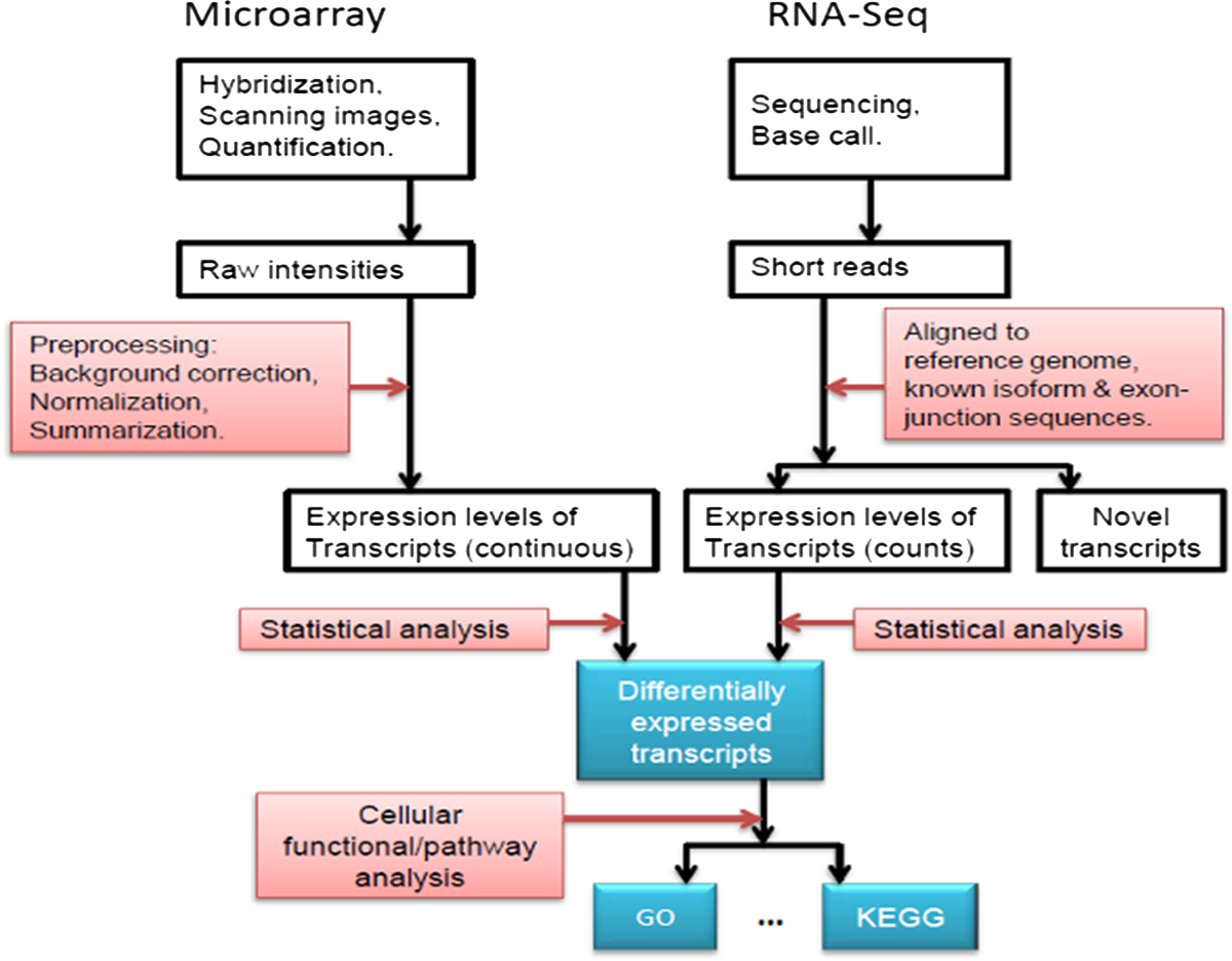
What’s measured. The abundance of each gene’s mRNA. A highly expressed gene has many mRNA copies; a silent gene has almost none. Two technologies measure this (Figure 9.3). The older, the microarray, is a glass chip dotted with short DNA probes, one set per gene; labelled mRNA from the sample sticks to its matching probe and the spot glows, brightly for abundant genes. The newer, RNA-seq, skips the chip: it sequences the mRNA directly and counts reads per gene. RNA-seq has largely replaced microarrays because it doesn’t need a probe designed in advance and measures a wider range of abundances, but enormous archives of microarray data remain valuable and reusable.
What the data look like. A matrix with one row per gene and one column per sample. Each entry is that gene’s expression in that sample — a fluorescence intensity (microarray) or a read count (RNA-seq). This is the single most common data shape in the book.
→ In this book. The SummarizedExperiment chapter builds the container that holds this matrix together with its gene and sample annotations. GEOquery downloads a real published expression dataset and runs a PCA on it. The k-means chapter clusters genes from a classic yeast microarray time course. Several machine-learning worked examples predict a label or a number from an expression matrix.
9.4.2 DNA methylation
The question. The DNA sequence is fixed, but cells can write reversible chemical annotations on top of it that change how genes behave. Where are those marks, and how do they shift with age, tissue, or disease?
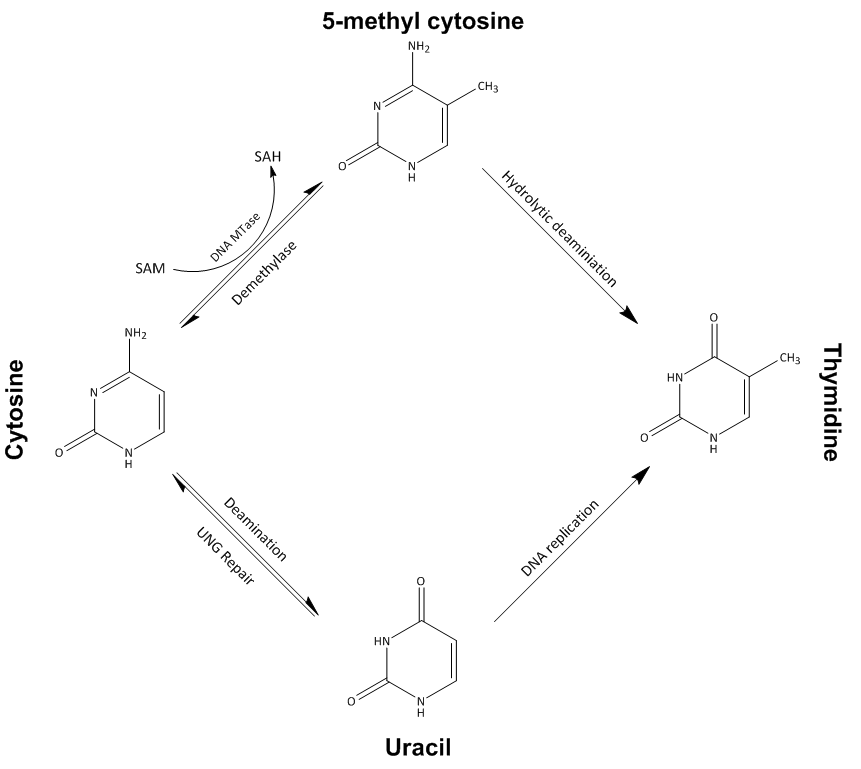
What’s measured. DNA methylation is the most studied such mark: a methyl group added to a cytosine (the “C” of the alphabet), almost always where a C sits next to a G — a so-called CpG site (Figure 9.4). Methylation in a gene’s promoter tends to switch the gene off, so the methylation pattern is part of how a cell remembers what type of cell it is. Specialized arrays (or sequencing) report, for each of hundreds of thousands of CpG sites, the fraction of DNA molecules that are methylated there — a number between 0 (never methylated) and 1 (always).
What the data look like. A matrix with one row per CpG site and one column per sample, each entry a methylation fraction between 0 and 1. Same features-by-samples shape as expression, just a different feature and a different unit.
→ In this book. The machine-learning worked example predicting age from DNA methylation trains an epigenetic clock: a model that reads a person’s age off the methylation values at age-sensitive CpG sites.
9.4.3 ChIP-seq: where proteins bind the genome
The question. Regulation is carried out by proteins that physically sit on the DNA — transcription factors at their target sites, and the modified histone proteins that mark active or silent regions. Where on the genome does a given protein bind?
What’s measured. ChIP-seq (chromatin immunoprecipitation followed by sequencing) uses an antibody to fish out just the DNA fragments that a chosen protein was attached to, then sequences them (Figure 9.5). Align those reads back to the genome and they pile up into peaks at the protein’s binding sites — and stay flat everywhere else. A peak says “the protein was here.”
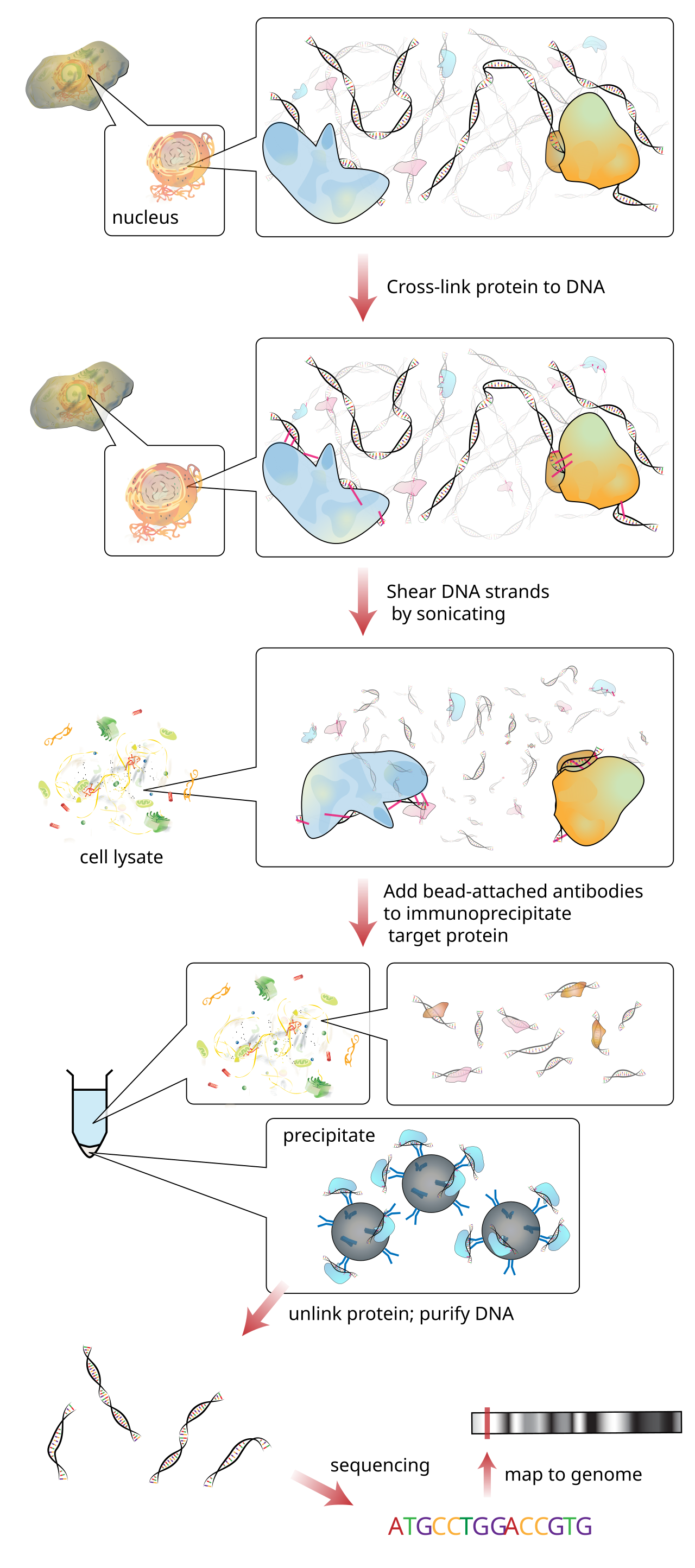
What the data look like. Not a dense matrix but a list of genomic intervals — each peak is a chromosome, a start, and an end, often with a score. This is a fundamentally positional kind of data, and handling it well is what Bioconductor’s genomic-ranges tools exist for.
→ In this book. The genomic ranges and features chapter teaches the interval operations (overlaps, nearest-feature, flanking) that turn peaks into biology, and the ChIP-seq peaks chapter loads a real set of CTCF ChIP-seq peaks from the ENCODE project and explores them. A machine-learning example even predicts gene expression from histone-mark ChIP-seq.
9.4.4 ATAC-seq: where the genome is open
The question. Before a gene can be switched on, the regulatory DNA around it has to be physically accessible — unwound from its nucleosome spools so that proteins can reach it. Which stretches of the genome are open in this cell type?
What’s measured. ATAC-seq uses an enzyme that can only cut DNA where it is exposed; it slices the accessible regions and tags them for sequencing in one step (Figure 9.6). Reads accumulate over open regions — active promoters, enhancers, transcription-factor sites — and are absent over the tightly packed, silent majority of the genome. As a bonus, the lengths of the sequenced fragments reveal where individual nucleosomes sit.
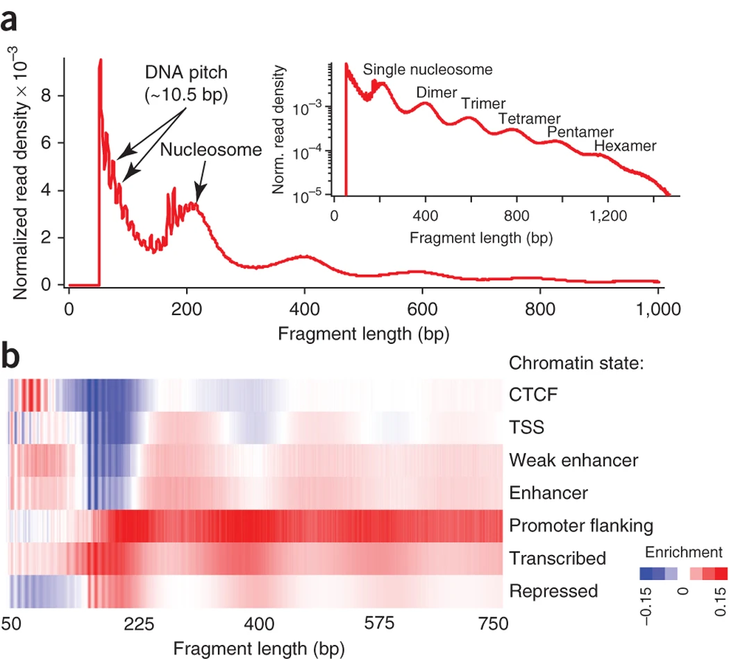
What the data look like. Like ChIP-seq, genomic intervals plus a coverage signal along the genome: peaks of accessibility, and a per-base pileup you can plot as a track. The same GRanges machinery handles both.
→ In this book. The ATAC-seq chapter takes real sequencing data and walks it from aligned reads to a biological picture: where reads pile up, how fragment length reveals nucleosome positions, and how accessibility lines up with the starts of genes.
9.4.5 Single-cell RNA-seq
The question. Bulk RNA-seq mashes a whole tissue into one tube and reports the average expression over every cell in it — blurring neurons, glia, and blood vessels into one indistinct smear. But a tissue is a mixture of cell types. Which cell types are present, in what proportions, and what makes each one distinct?
What’s measured. Single-cell RNA-seq (scRNA-seq) measures gene expression one cell at a time (Figure 9.7). Clever microfluidics isolate tens of thousands of individual cells, tag each cell’s RNA with a unique molecular barcode, and sequence them all together; the barcode lets you sort the reads back to the cell they came from. Instead of one average profile you get a catalog of thousands of individual profiles.
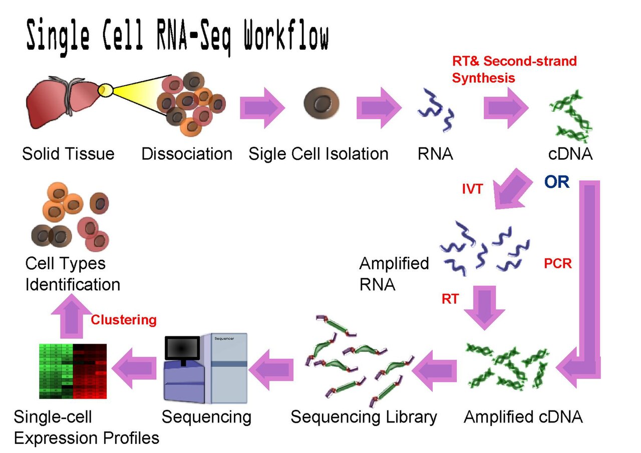
What the data look like. A matrix with one row per gene and one column per cell — the same shape as bulk expression, but now with tens of thousands of columns and mostly zeros (any one cell expresses only a fraction of all genes). That scale and sparsity drive the whole analysis: normalize, reduce to a 2-D map, cluster the cells, and label the clusters by their marker genes.
→ In this book. The single-cell RNA-seq chapter takes a published mouse-brain dataset from raw counts to a labelled map of cell types, using the standard load → normalize → reduce → cluster → annotate workflow.
9.4.6 The microbiome: 16S and metagenomic sequencing
The question. Your gut, skin, and mouth host vast communities of bacteria and other microbes that influence digestion, immunity, and disease. Which microbes are present in a sample, and in what proportions — and how do those proportions differ between healthy and sick people?
What’s measured. Rather than sequence every microbe’s whole genome, the most common approach amplifies and sequences a single marker gene — the 16S ribosomal RNA gene — that every bacterium carries but whose sequence varies just enough between species to act as a barcode (Figure 9.8). Counting how many reads match each barcode tells you how abundant each microbe is. (The more exhaustive alternative, shotgun metagenomics, sequences all the DNA in the sample at once.)
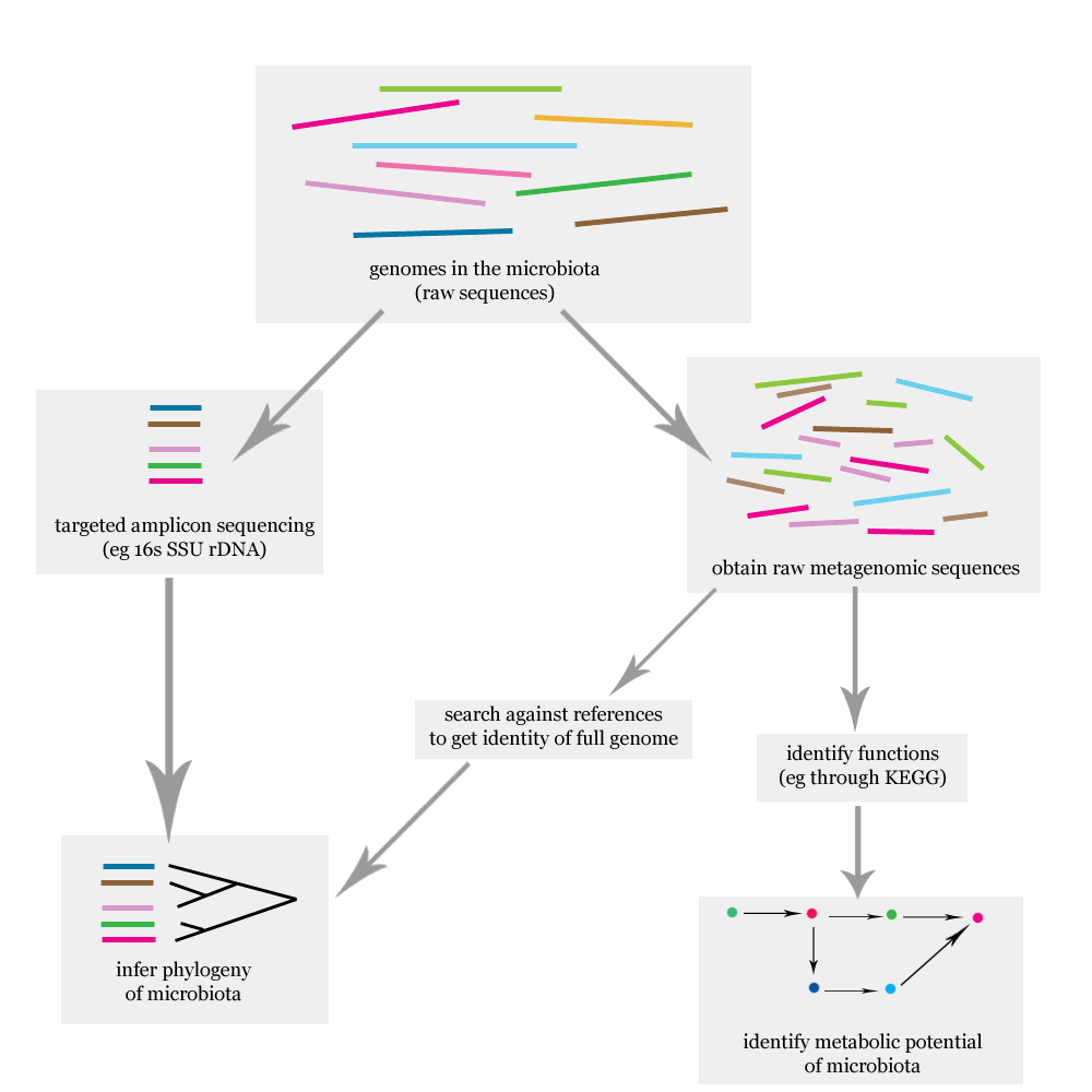
What the data look like. A table with one row per microbe (taxon) and one column per sample, each entry an abundance — again the features-by-samples shape, often paired with a tree describing how the taxa are evolutionarily related.
→ In this book. The microbiome chapter loads a curated gut-microbiome dataset from a colorectal-cancer study and asks how diverse each sample is, whether patients and controls separate, and which microbes dominate — all from a TreeSummarizedExperiment that bundles the abundance table with that evolutionary tree.
9.5 How the assays connect
Step back and the pattern is clear: a handful of biological questions, the same counting trick under most of them, and just two data shapes — a dense features-by-samples matrix, or a list of genomic intervals (Table 9.1).
| Assay | Biological question | What’s measured | Data shape | Chapter |
|---|---|---|---|---|
| Gene expression | Which genes are on, how strongly? | mRNA abundance per gene | genes × samples matrix | SummarizedExperiment, GEOquery, k-means |
| DNA methylation | Where is DNA chemically marked? | methylation fraction per CpG | CpG sites × samples matrix | Methylation age |
| ChIP-seq | Where does a protein bind? | read pileup at binding sites | list of genomic intervals (peaks) | Genomic ranges, Histone marks |
| ATAC-seq | Where is the genome open? | accessibility signal | intervals + coverage | ATAC-seq |
| scRNA-seq | Expression per cell; which cell types? | mRNA per gene, per cell | genes × cells matrix | Single-cell |
| Microbiome (16S) | Which microbes, in what proportions? | abundance per taxon | taxa × samples table (+ tree) | Microbiome |
Once you can place an unfamiliar experiment into this table — what was put in the tube, what got counted, what shape is the result — the analysis chapters become much easier to follow, because they are all variations on handling one of these two data shapes.
9.6 Exercises
These are reading-comprehension questions; no R required. Try to answer before opening the solution.
Same shape, different meaning. A microbiome abundance table and a bulk RNA-seq dataset both arrive as a features-by-samples matrix. What does a single row represent in each case, and what does a single number mean?
NoteSolutionIn RNA-seq, a row is a gene and a number is that gene’s expression (a read count or intensity) in one sample. In the microbiome table, a row is a microbe (taxon) and a number is that taxon’s abundance in one sample. The container is identical — which is exactly why both use
SummarizedExperiment-style objects — but the biological meaning of rows and values is completely different.Matrix or intervals? For each experiment, say whether the natural output is a dense features-by-samples matrix or a list of genomic intervals:
- measuring how strongly 20,000 genes are expressed across 50 tumors;
- finding every place the CTCF protein binds the genome;
- mapping which regions of DNA are accessible in a cell type.
NoteSolution- is a matrix (genes × samples). (b) and (c) are lists of genomic intervals — ChIP-seq peaks and ATAC-seq accessible regions are both positional, which is why both are handled with
GRanges.
What went in the tube? RNA-seq, ChIP-seq, ATAC-seq, and 16S microbiome sequencing all run on the same kind of sequencer and all end in counting reads. In one sentence each, what makes them different experiments?
NoteSolutionThey differ in what is put into the sequencing library: all the mRNA in the sample (RNA-seq), only the DNA a chosen protein was bound to (ChIP-seq), only the accessible DNA (ATAC-seq), or an amplified marker gene such as 16S (microbiome). Same machine and same counting step; different molecules going in, so different questions answered.
Why bother with single cells? A colleague has bulk RNA-seq from a brain sample and asks why anyone would pay more to do single-cell RNA-seq on the same tissue. Give the one-sentence reason.
NoteSolutionBulk RNA-seq reports the average expression over all cells, blurring together the distinct cell types in the tissue; single-cell RNA-seq measures each cell separately, so it can reveal which cell types are present and how they differ — including rare populations the average would hide.
9.7 Summary
You now have the mental model the rest of the book assumes. You can explain the central dogma (DNA → RNA → protein) and why measuring RNA tells you which genes are on. You know the unifying trick behind most modern assays — sequence millions of fragments and count where they come from — and that the assays differ mainly in what goes into the tube. And for each of the six assays in this book you can name the biological question it answers and the shape of data it produces: a features-by-samples matrix for expression, methylation, single-cell, and microbiome data; a list of genomic intervals for ChIP-seq and ATAC-seq. When a later chapter opens with “a matrix of counts” or “a set of peaks,” you’ll know exactly what it means and where it came from.
9.8 Resources
- Central dogma — NHGRI genetics glossary, with a short narrated explainer.
- The Gene Expression Omnibus (GEO) — the public archive the book draws several datasets from; browsing a few entries is a good way to see these assays “in the wild.”
- EMBL-EBI training — free, accessible introductions to RNA-seq, ChIP-seq, single-cell, and more, if you want a deeper but still gentle treatment of any assay above.