5 Packages, simulation, and the law of large numbers

Author

Affiliation

University of Colorado
Anschutz School of Medicine

Published

June 1, 2024

Modified

June 23, 2026

In the previous chapter we built random_sequence(), a tiny generative model that spits out random DNA. We claimed each base is equally likely. But is it? And what does a collection of these sequences actually look like? When you can’t answer a question by staring at code, two general-purpose tools come to the rescue, and you’ll use them together for the rest of your career:

Simulation — generate the data many times over and look at the results in aggregate, and
Visualization — draw a picture so the pattern jumps out.

Simulation we can do with base R. Visualization, in the style this book uses, needs a package — so that’s where we start.

5.1 What you’ll learn

Install and load R packages, and tell those two steps apart.
Reduce a whole dataset to a single number — a statistic — and write a function that computes one.
Repeat a random experiment many times with replicate().
Visualize the spread of a statistic with a histogram (using ggplot2).
State and see the law of large numbers: more data means a statistic settles toward its expected value.

5.2 Packages

R on its own is powerful, but most of what makes it indispensable lives in packages: bundles of functions, data, and documentation that other people have written and shared. Rather than coding a histogram routine from scratch, you load a package that already has one — well-tested, documented, and used by thousands.

5.2.1 Installing vs. loading

There are two distinct steps, and conflating them is the single most common beginner stumble.

Installing downloads a package onto your computer. You do it once (per machine, per major update). Most packages come from CRAN, the central R package repository:

install.packages("ggplot2")

For bioinformatics packages you’ll instead use Bioconductor, whose installer, BiocManager, can also install regular CRAN packages. You install BiocManager itself just once:

install.packages("BiocManager")
BiocManager::install("ggplot2")

Loading makes an installed package’s functions available in your current R session. You do it every session, with library():

library(ggplot2)

After that line, ggplot2’s functions are in scope and ready to use.

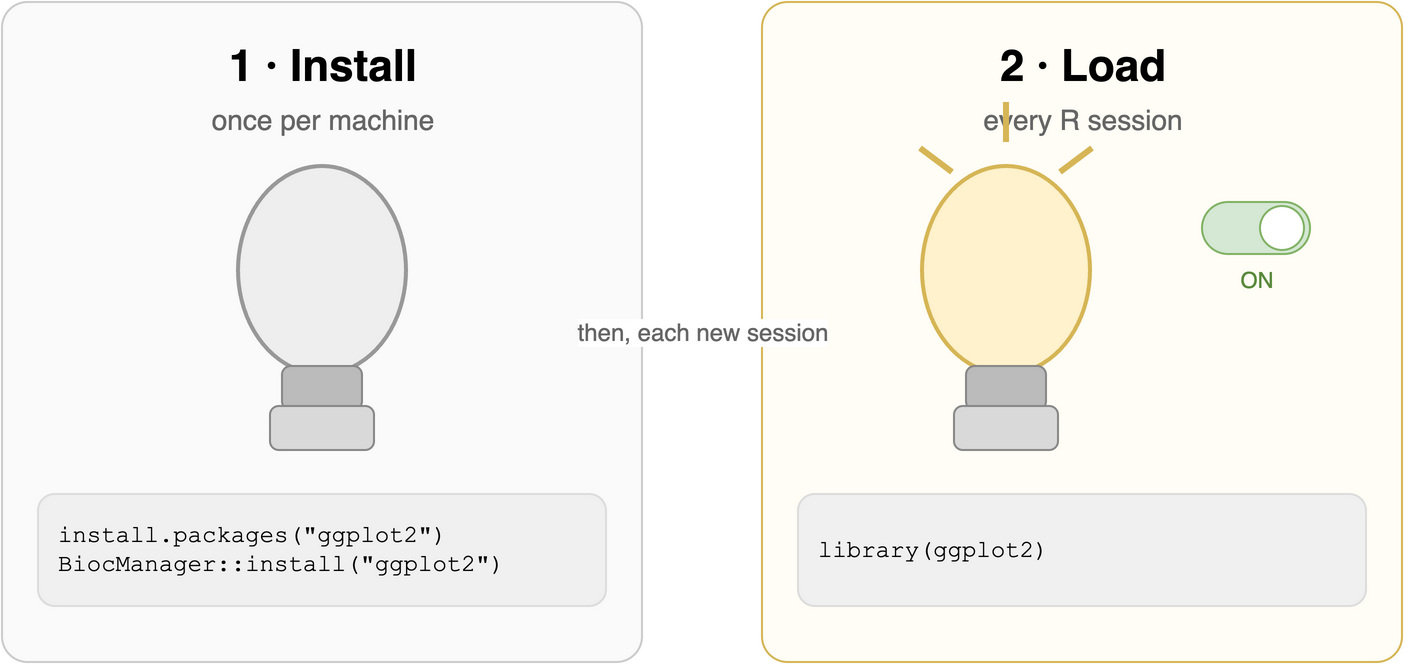
Figure 5.1: Installing versus loading a package. **Installing** (`install.packages()` or `BiocManager::install()`) puts the package on your machine — like screwing a light bulb into its socket, you do it once and it stays. **Loading** it with `library()` is flicking the switch on — you do it every time you want the light, in every new R session, because R forgets its loaded packages when you quit.

Install once, load every time

As in Figure 5.1, you install a package once per machine, then load it with library() in every session that needs it. That’s why library() calls live at the top of your scripts and Quarto documents — they re-light the bulb each time.

5.3 A statistic: one number that summarizes many

Our generative model claims A, C, G, and T are equally likely. A natural way to check is GC content: the fraction of a sequence’s bases that are G or C. It’s a real and useful quantity — GC content varies systematically across organisms and across regions of a genome — and it’s a perfect first example of a statistic.

A statistic is just a single number computed from data that summarizes some aspect of it. The mean of a set of measurements is a statistic; so is GC content. Statistics take a pile of numbers you can’t hold in your head and boil it down to something you can.

Let’s write a function for it. We can reuse the %in% idea and the trick that the mean of a logical vector is the fraction of TRUEs (see the Vectors chapter):

gc_content <- function(sequence) {
  bases <- strsplit(sequence, "")[[1]]   # split the string into single letters
  mean(bases %in% c("G", "C"))           # fraction of bases that are G or C
}

We also need our generator from last chapter. Each chapter stands on its own, so let’s redefine both pieces here:

nucleotides <- c("A", "C", "G", "T")

random_sequence <- function(n = 100, prob = NULL) {
  bases <- sample(nucleotides, size = n, replace = TRUE, prob = prob)
  paste(bases, collapse = "")
}

Now compute the GC content of a single random sequence:

seq1 <- random_sequence(n = 100)
gc_content(seq1)

[1] 0.46

You’ll get something near 0.5, but probably not exactly — randomness wobbles. Run it on another sequence and the number changes:

gc_content(random_sequence(n = 100))

[1] 0.49

gc_content(random_sequence(n = 100))

[1] 0.47

A single statistic from a single sequence doesn’t tell us much, precisely because it jumps around. To see the real behavior of our model, we need many sequences.

5.4 Repeating an experiment with `replicate()`

The replicate() function runs an expression many times and collects the results into a vector. Read it as “do this n times and give me back all the answers.” Here we generate 1000 sequences and record the GC content of each:

gc_values <- replicate(1000, gc_content(random_sequence(n = 100)))
length(gc_values)

[1] 1000

head(gc_values)

[1] 0.60 0.54 0.57 0.49 0.51 0.51

gc_values is now a vector of 1000 statistics — one experiment’s worth of evidence about how our model behaves. Summaries help, but a picture helps more.

5.5 Visualizing the spread

A histogram bins the values and draws a bar for how many fell in each bin, revealing the shape of the distribution. With ggplot2 we describe the plot in layers: the data, an aesthetic mapping (which variable goes on the x-axis), and a geometry (here, a histogram).

library(ggplot2)

ggplot(data.frame(gc = gc_values), aes(x = gc)) +
  geom_histogram(binwidth = 0.02, fill = "steelblue", color = "white") +
  labs(x = "GC content", y = "Number of sequences")

Figure 5.2: Distribution of GC content across 1000 simulated 100-base sequences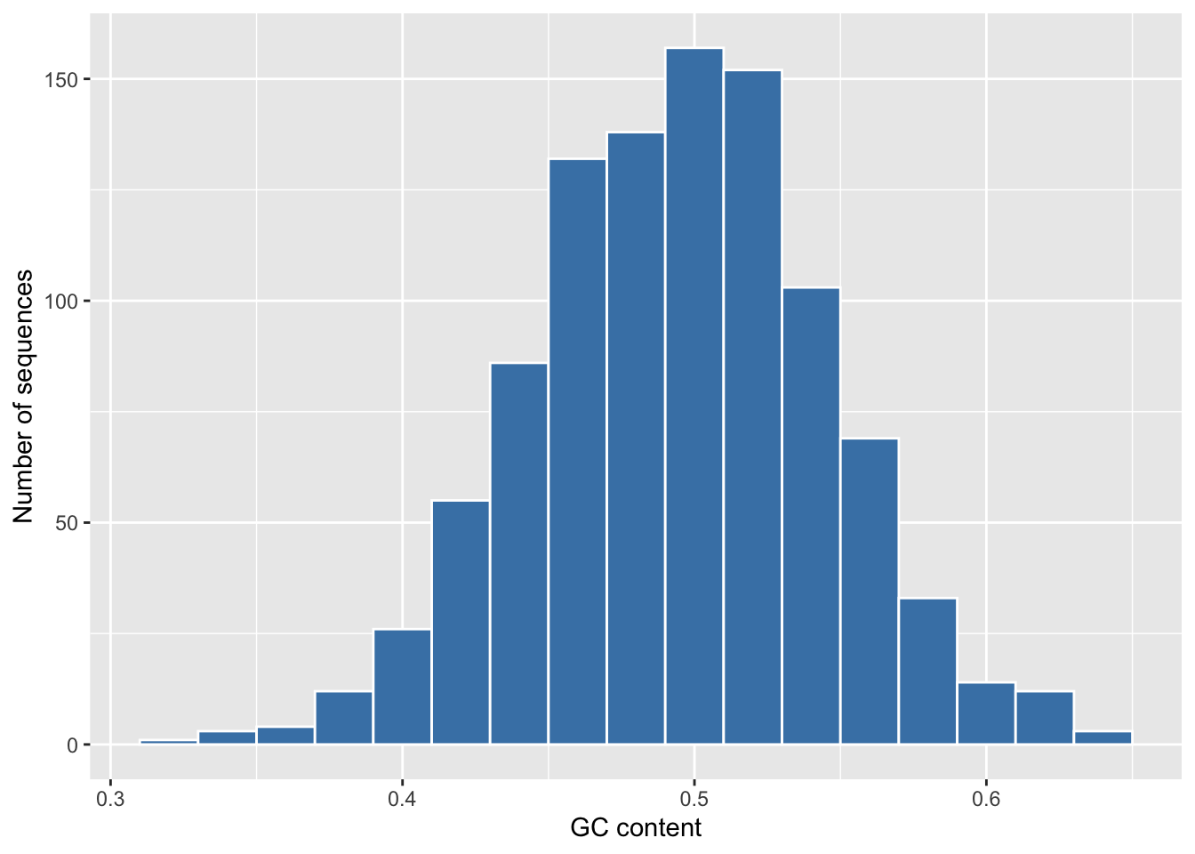. The values cluster around 0.5, the expected GC content when all four bases are equally likely.

The values pile up around 0.5 — just as they should when every base is equally likely — and fan out symmetrically on either side. That spread is the randomness in our model made visible. (If qplot() is what you learned years ago, note that it’s now deprecated; ggplot() + geom_histogram() is the current idiom, and the ggplot2 chapter builds it up properly.)

5.6 The law of large numbers

Here is the payoff. Each sequence’s GC content is itself an average — the fraction of G/C over the bases in that sequence. What happens to that average as we put more data into each sequence, i.e. make the sequences longer?

Let’s compute GC content for sequences of three different lengths, many times each, and compare the spreads:

gc_by_length <- rbind(
  data.frame(length = "25",   gc = replicate(1000, gc_content(random_sequence(25)))),
  data.frame(length = "100",  gc = replicate(1000, gc_content(random_sequence(100)))),
  data.frame(length = "1000", gc = replicate(1000, gc_content(random_sequence(1000))))
)
gc_by_length$length <- factor(gc_by_length$length, levels = c("25", "100", "1000"))

ggplot(gc_by_length, aes(x = gc)) +
  geom_histogram(binwidth = 0.01, fill = "steelblue", color = "white") +
  facet_wrap(~ length, ncol = 1) +
  labs(x = "GC content", y = "Number of sequences")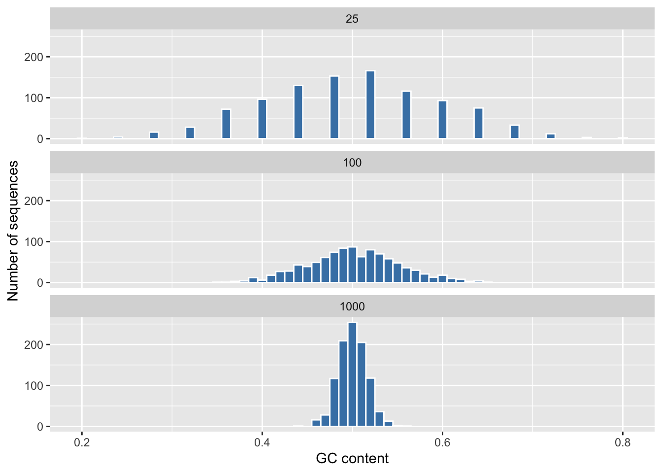

Figure 5.3: GC content for sequences of length 25, 100, and 1000 (1000 sequences each). As sequence length grows, the distribution of the statistic tightens around its expected value of 0.5 — the law of large numbers in action.

The center stays put at 0.5, but the spread shrinks dramatically as the sequences get longer. A 25-base sequence can easily land at 0.3 or 0.7 by chance; a 1000-base sequence almost never strays far from 0.5. More data, less wobble.

That is the law of large numbers: as you average over more and more independent observations, the average converges toward the true expected value, and the chance of a large deviation shrinks toward zero. Our expected GC content is 0.5 (G and C are two of four equally likely bases), and longer sequences hug that value ever more tightly.

What the law does and doesn’t promise

The law of large numbers is about the average, not the individual draws. Single bases never stop being random — extend a sequence and each new base is still a coin-flip for G/C. What stabilizes is the fraction over the whole sequence. And the convergence relies on our independence assumption from the last chapter; in real DNA, where neighboring bases are correlated, the expected GC content is still meaningful, but the simple “spread shrinks like this” arithmetic no longer applies cleanly.

5.7 Changing the model: GC-rich and GC-poor genomes

Expected GC content of 0.5 was a consequence of our equal-probability assumption. Real organisms span a wide range — the Plasmodium falciparum genome is about 80% AT, while some Streptomyces exceed 70% GC. Our prob argument lets us model that. Weight G and C four times as heavily as A and T and the whole distribution slides toward high GC:

gc_rich <- replicate(
  1000,
  gc_content(random_sequence(n = 100, prob = c(1, 4, 4, 1)))  # A, C, G, T
)

ggplot(data.frame(gc = gc_rich), aes(x = gc)) +
  geom_histogram(binwidth = 0.02, fill = "darkorange", color = "white") +
  labs(x = "GC content", y = "Number of sequences")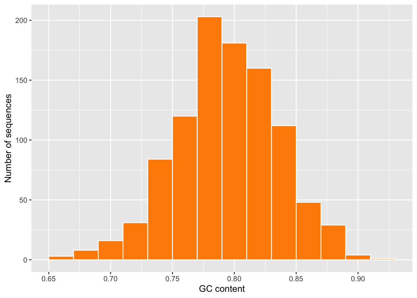

Figure 5.4: GC content of 1000 simulated GC-rich sequences (G and C weighted 4x relative to A and T). The distribution now centers near 0.8 rather than 0.5 — the expected value tracks the probabilities you put into the model.

The peak moves to roughly 0.8, exactly where the weights predict (the combined probability of G or C is 8/10). The expected value of a statistic is set by the model’s assumptions — change the assumptions and the statistic follows.

5.8 Exercises

Write a one-line expression (no new function) that computes the mean GC content over 500 sequences of length 200.
NoteSolution
mean(replicate(500, gc_content(random_sequence(200))))

[1] 0.49864
replicate() gathers 500 statistics into a vector and mean() reduces that vector to one number — a statistic computed from other statistics.
Without running it, predict whether the histogram for length-2000 sequences would be wider or narrower than the length-1000 one in Figure 5.3. Why?

NoteSolution

Narrower. The law of large numbers says more data per sequence means less spread in the average, so doubling the length tightens the distribution further around 0.5.
Use prob to build a strongly AT-rich generator (like Plasmodium), simulate 1000 sequences of length 100, and report the approximate center of their GC-content distribution.
NoteSolution
at_rich <- replicate( 1000, gc_content(random_sequence(n = 100, prob = c(4, 1, 1, 4))) # A, C, G, T ) mean(at_rich)

[1] 0.19793
Weighting A and T four times as heavily puts the combined G/C probability at 2/10, so GC content centers near 0.2.
library() errors with “there is no package called ‘ggplot2’” on a fresh machine. What step was skipped, and what’s the one-line fix?

NoteSolution

The package was never installed on that machine. Run install.packages("ggplot2") (or BiocManager::install("ggplot2")) once, then library(ggplot2) will work in every session afterward.

5.9 Summary

You now have the simulation-and-visualization loop that underlies a huge amount of practical statistics:

Packages extend R. Install them once (install.packages() / BiocManager::install()) and load them every session (library()).
A statistic is a single number summarizing data; GC content is ours, and a few lines of R turn it into a reusable function.
replicate() runs a random experiment many times, and a histogram shows how the resulting statistic is distributed.
The law of large numbers says a statistic computed from more data clusters more tightly around its expected value — visible as the shrinking spread in Figure 5.3 — and that expected value is determined by the assumptions baked into your model.

These same two tools — repeat it many times, then look at the distribution — return in the statistics and machine-learning chapters, where the “experiment” is a real analysis rather than a string of random bases.