34 Genomic ranges and features

Author

Affiliation

University of Colorado
Anschutz School of Medicine

Published

June 1, 2024

Modified

June 11, 2026

Almost everything you study in genomics lives at a place on the genome. A gene sits between two coordinates on a chromosome. An exon is a stretch within that gene. A ChIP-seq peak marks where a protein bound. A SNP is a single position. As soon as you have two such sets of places, the most interesting biological questions become questions about location: Which peaks fall inside a promoter? What is the nearest gene to this variant? Where do these two experiments agree?

In this chapter you’ll learn to represent those places as genomic ranges and to ask how they relate to one another. The workhorse is Bioconductor’s GenomicRanges package (Lawrence et al. 2013), which gives you a compact object to hold ranges plus any data attached to them, and a vocabulary of fast operations — overlap, nearest-neighbor, flank, reduce — that scale to millions of regions. We’ll build small example objects by hand so you can see exactly what each operation does, then finish with real gene models pulled from a genome annotation.

A note on coordinate systems

Different tools count positions differently. The UCSC Genome Browser uses 0-based, half-open coordinates internally, while Ensembl and Bioconductor use 1-based, inclusive coordinates (position 1 is the first base, and both endpoints are included). GRanges objects are always 1-based and inclusive, which is one fewer thing to track once you stay inside Bioconductor.

34.1 What you’ll learn

Build a GRanges object and read its two-part display (coordinates on the left, metadata on the right).
Subset and extract parts of a GRanges object with accessors like seqnames(), ranges(), strand(), and mcols().
Apply intra-range operations (flank(), shift(), resize()) and inter-range operations (reduce(), disjoin(), gaps(), coverage()).
Find relationships between two sets of ranges with findOverlaps(), subsetByOverlaps(), nearest(), and distanceToNearest().
Group ranges into a GRangesList (for example, the exons of a transcript).
Pull gene, transcript, and exon models out of a TxDb annotation package.

34.2 Bioconductor and GenomicRanges

library(GenomicRanges)

The Bioconductor GenomicRanges package (Lawrence et al. 2013) gives you the GRanges container for genomic intervals together with a vocabulary of fast operations on them — subsetting, resizing, overlap, nearest-neighbor, and genome arithmetic. The rest of this chapter introduces both by example, building small objects by hand so you can see exactly what each operation does.

GRanges is built on R’s S4 class system, so each object carries dedicated slots — seqnames, ranges, strand, and metadata — with methods that operate on them. Three related containers show up throughout the chapter:

Class	What it holds	Typical use
`GRanges`	a set of genomic ranges plus metadata	ChIP-seq peaks, CpG islands, genes
`GRangesList`	a list of `GRanges` objects	exons grouped by transcript
`IRanges`	plain integer ranges	the building block inside a `GRanges`

Table 34.1: The containers used in this chapter.

A compact cheat-sheet of the accessor and operation methods is collected under Quick reference at the end of the chapter; we meet each one in context first.

To get going, we can construct a GRanges object by hand as an example.

The GRanges class represents a collection of genomic ranges that each have a single start and end location on the genome. It can be used to store the location of genomic features such as contiguous binding sites, transcripts, and exons. These objects can be created by using the GRanges constructor function. The following code creates one from scratch. (The Rle() calls in it simply repeat each value a given number of times — a compact “run-length” shorthand we return to under coverage later.)

gr <- GRanges(
    seqnames = Rle(c("chr1", "chr2", "chr1", "chr3"), c(1, 3, 2, 4)),
    ranges = IRanges(101:110, end = 111:120, names = head(letters, 10)),
    strand = Rle(strand(c("-", "+", "*", "+", "-")), c(1, 2, 2, 3, 2)),
    score = 1:10,
    GC = seq(1, 0, length=10))
gr

GRanges object with 10 ranges and 2 metadata columns:
    seqnames    ranges strand |     score        GC
       <Rle> <IRanges>  <Rle> | <integer> <numeric>
  a     chr1   101-111      - |         1  1.000000
  b     chr2   102-112      + |         2  0.888889
  c     chr2   103-113      + |         3  0.777778
  d     chr2   104-114      * |         4  0.666667
  e     chr1   105-115      * |         5  0.555556
  f     chr1   106-116      + |         6  0.444444
  g     chr3   107-117      + |         7  0.333333
  h     chr3   108-118      + |         8  0.222222
  i     chr3   109-119      - |         9  0.111111
  j     chr3   110-120      - |        10  0.000000
  -------
  seqinfo: 3 sequences from an unspecified genome; no seqlengths

This creates a GRanges object with 10 genomic ranges. The output of the GRanges show() method separates the information into a left and right hand region that are separated by | symbols (see Figure 34.1). The genomic coordinates (seqnames, ranges, and strand) are located on the left-hand side and the metadata columns are located on the right. For this example, the metadata is comprised of score and GC information, but almost anything can be stored in the metadata portion of a GRanges object.

Reading a GRanges: the | is the dividing line

Think of a GRanges as a spreadsheet with a heavy vertical rule drawn down the middle. Everything to the left of the | answers “where?” — the chromosome (seqnames), the start and end (ranges), and the strand. These columns are mandatory and have their own special accessors. Everything to the right of the | answers “what do we know about it?” — the metadata: scores, GC content, gene names, p-values, whatever you attach. These are optional and you reach them all at once with mcols(). Keeping that line in mind makes every later operation easier: range operations rearrange the left side; your annotations ride along on the right.

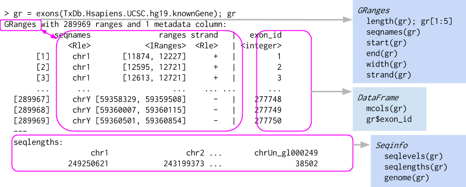
Figure 34.1: The structure of a `GRanges` object, which behaves a bit like a vector of ranges, although the analogy is not perfect. A `GRanges` object is composed of the “Ranges” part the lefthand box, the “metadata” columns (the righthand box), and a “seqinfo” part that describes the names and lengths of associated sequences. Only the “Ranges” part is required. The figure also shows a few of the “accessors” and approaches to subsetting a `GRanges` object.

The components of the genomic coordinates within a GRanges object can be extracted using the seqnames, ranges, and strand accessor functions.

seqnames(gr)

factor-Rle of length 10 with 4 runs
  Lengths:    1    3    2    4
  Values : chr1 chr2 chr1 chr3
Levels(3): chr1 chr2 chr3

ranges(gr)

IRanges object with 10 ranges and 0 metadata columns:
        start       end     width
    <integer> <integer> <integer>
  a       101       111        11
  b       102       112        11
  c       103       113        11
  d       104       114        11
  e       105       115        11
  f       106       116        11
  g       107       117        11
  h       108       118        11
  i       109       119        11
  j       110       120        11

strand(gr)

factor-Rle of length 10 with 5 runs
  Lengths: 1 2 2 3 2
  Values : - + * + -
Levels(3): + - *

Note that the GRanges object has information to the “left” side of the | that has special accessors. The information to the right side of the |, when it is present, is the metadata and is accessed using mcols(), for “metadata columns”.

class(mcols(gr))

[1] "DFrame"
attr(,"package")
[1] "S4Vectors"

mcols(gr)

DataFrame with 10 rows and 2 columns
      score        GC
  <integer> <numeric>
a         1  1.000000
b         2  0.888889
c         3  0.777778
d         4  0.666667
e         5  0.555556
f         6  0.444444
g         7  0.333333
h         8  0.222222
i         9  0.111111
j        10  0.000000

Since the class of mcols(gr) is DFrame, we can use the DataFrame (Bioconductor’s data-frame-like table) approaches to work with the data.

mcols(gr)$score

 [1]  1  2  3  4  5  6  7  8  9 10

We can even assign a new column. Here we add an AT column derived from GC (since the fractions sum to 1). Notice that the new column appears on the right of the |, alongside score and GC.

mcols(gr)$AT <- 1 - mcols(gr)$GC
gr

GRanges object with 10 ranges and 3 metadata columns:
    seqnames    ranges strand |     score        GC        AT
       <Rle> <IRanges>  <Rle> | <integer> <numeric> <numeric>
  a     chr1   101-111      - |         1  1.000000  0.000000
  b     chr2   102-112      + |         2  0.888889  0.111111
  c     chr2   103-113      + |         3  0.777778  0.222222
  d     chr2   104-114      * |         4  0.666667  0.333333
  e     chr1   105-115      * |         5  0.555556  0.444444
  f     chr1   106-116      + |         6  0.444444  0.555556
  g     chr3   107-117      + |         7  0.333333  0.666667
  h     chr3   108-118      + |         8  0.222222  0.777778
  i     chr3   109-119      - |         9  0.111111  0.888889
  j     chr3   110-120      - |        10  0.000000  1.000000
  -------
  seqinfo: 3 sequences from an unspecified genome; no seqlengths

Another common way to create a GRanges object is to start with a data.frame, perhaps created by hand like below or read in using read.csv or read.table. We can convert from a data.frame, when columns are named appropriately, to a GRanges object.

df_regions <- data.frame(chromosome = rep("chr1", 10),
                         start = seq(1000, 10000, 1000),
                         end = seq(1100, 10100, 1000))
as(df_regions, 'GRanges') # note that names have to match with GRanges slots

GRanges object with 10 ranges and 0 metadata columns:
       seqnames      ranges strand
          <Rle>   <IRanges>  <Rle>
   [1]     chr1   1000-1100      *
   [2]     chr1   2000-2100      *
   [3]     chr1   3000-3100      *
   [4]     chr1   4000-4100      *
   [5]     chr1   5000-5100      *
   [6]     chr1   6000-6100      *
   [7]     chr1   7000-7100      *
   [8]     chr1   8000-8100      *
   [9]     chr1   9000-9100      *
  [10]     chr1 10000-10100      *
  -------
  seqinfo: 1 sequence from an unspecified genome; no seqlengths

## fix column name
colnames(df_regions)[1] <- 'seqnames'
gr2 <- as(df_regions, 'GRanges')
gr2

GRanges object with 10 ranges and 0 metadata columns:
       seqnames      ranges strand
          <Rle>   <IRanges>  <Rle>
   [1]     chr1   1000-1100      *
   [2]     chr1   2000-2100      *
   [3]     chr1   3000-3100      *
   [4]     chr1   4000-4100      *
   [5]     chr1   5000-5100      *
   [6]     chr1   6000-6100      *
   [7]     chr1   7000-7100      *
   [8]     chr1   8000-8100      *
   [9]     chr1   9000-9100      *
  [10]     chr1 10000-10100      *
  -------
  seqinfo: 1 sequence from an unspecified genome; no seqlengths

The first as() call worked even though the chromosome column was named chromosome — as() recognized start and end and treated the rest as metadata. After we rename that column to seqnames, the conversion places it correctly on the left of the | as the sequence name.

GRanges have one-dimensional-like behavior. For instance, we can check the length and even give GRanges names.

names(gr)

 [1] "a" "b" "c" "d" "e" "f" "g" "h" "i" "j"

length(gr)

[1] 10

34.2.1 Subsetting GRanges objects

While GRanges objects look a bit like a data.frame, they can be thought of as vectors with associated ranges. Subsetting, then, works very similarly to vectors. To subset a GRanges object to include only second and third regions:

gr[2:3]

GRanges object with 2 ranges and 3 metadata columns:
    seqnames    ranges strand |     score        GC        AT
       <Rle> <IRanges>  <Rle> | <integer> <numeric> <numeric>
  b     chr2   102-112      + |         2  0.888889  0.111111
  c     chr2   103-113      + |         3  0.777778  0.222222
  -------
  seqinfo: 3 sequences from an unspecified genome; no seqlengths

That said, if the GRanges object has metadata columns, we can also treat it like a two-dimensional object kind of like a data.frame. Note that the information to the left of the | is not like a data.frame, so we cannot do something like gr$seqnames. Here is an example of subsetting with the subset of one metadata column.

gr[2:3, "GC"]

GRanges object with 2 ranges and 1 metadata column:
    seqnames    ranges strand |        GC
       <Rle> <IRanges>  <Rle> | <numeric>
  b     chr2   102-112      + |  0.888889
  c     chr2   103-113      + |  0.777778
  -------
  seqinfo: 3 sequences from an unspecified genome; no seqlengths

The usual head() and tail() also work just fine.

head(gr,n=2)

GRanges object with 2 ranges and 3 metadata columns:
    seqnames    ranges strand |     score        GC        AT
       <Rle> <IRanges>  <Rle> | <integer> <numeric> <numeric>
  a     chr1   101-111      - |         1  1.000000  0.000000
  b     chr2   102-112      + |         2  0.888889  0.111111
  -------
  seqinfo: 3 sequences from an unspecified genome; no seqlengths

tail(gr,n=2)

GRanges object with 2 ranges and 3 metadata columns:
    seqnames    ranges strand |     score        GC        AT
       <Rle> <IRanges>  <Rle> | <integer> <numeric> <numeric>
  i     chr3   109-119      - |         9  0.111111  0.888889
  j     chr3   110-120      - |        10  0.000000  1.000000
  -------
  seqinfo: 3 sequences from an unspecified genome; no seqlengths

34.2.2 Interval operations on one GRanges object

34.2.2.1 Intra-range methods

The methods described in this section work one-region-at-a-time and are, therefore, called “intra-range” methods. Methods that work across all regions are described below in the Inter-range methods section.

To make the operations in this section easy to see, we’ll work with a small set of ranges on a single chromosome and draw a picture of each operation as we go. Here is the toy GRanges, g:

g <- GRanges("chr1",
             IRanges(start = c(5, 15, 30, 33, 50),
                     end   = c(22, 27, 42, 55, 58)),
             score = c(5, 8, 3, 9, 6))
names(g) <- letters[1:5]
g

GRanges object with 5 ranges and 1 metadata column:
    seqnames    ranges strand |     score
       <Rle> <IRanges>  <Rle> | <numeric>
  a     chr1      5-22      * |         5
  b     chr1     15-27      * |         8
  c     chr1     30-42      * |         3
  d     chr1     33-55      * |         9
  e     chr1     50-58      * |         6
  -------
  seqinfo: 1 sequence from an unspecified genome; no seqlengths

All five ranges are left unstranded (*) on purpose: the operations below act purely on position, which is the cleaner first mental model. We bring strand back in deliberately when it changes the answer — for flank() and resize().

The figures are all drawn with one small helper built on ggplot2. You don’t need to study it to follow the chapter — it just lays each range out as a labelled bar on a coordinate axis, stacking ranges into rows so overlapping ones stay visible — but it’s here if you’d like to reuse it.

Show the range-plotting helper

library(ggplot2)
library(patchwork)

# Lay a GRanges out as labelled bars on a shared coordinate axis. Overlapping
# ranges are stacked into separate rows with IRanges::disjointBins(); strand, when
# present, is shown by colour and unstranded (*) ranges are drawn grey.
plot_ranges <- function(gr, title = NULL, xlim = NULL) {
  bins <- as.integer(IRanges::disjointBins(ranges(gr)))
  df <- data.frame(
    xmin = start(gr) - 0.5, xmax = end(gr) + 0.5, lane = bins,
    strand = factor(as.character(strand(gr)), levels = c("+", "-", "*")),
    label = if (!is.null(names(gr))) names(gr) else as.character(seq_along(gr)))
  if (is.null(xlim)) xlim <- c(min(df$xmin), max(df$xmax))
  has_strand <- any(as.character(strand(gr)) %in% c("+", "-"))
  ggplot(df) +
    geom_rect(aes(xmin = xmin, xmax = xmax, ymin = lane - 0.35, ymax = lane + 0.35,
                  fill = strand), colour = "grey20", linewidth = 0.3) +
    geom_text(aes(x = (xmin + xmax) / 2, y = lane, label = label), size = 3.2) +
    scale_fill_manual(values = c("+" = "#4C72B0", "-" = "#C44E52", "*" = "grey80"),
                      drop = FALSE, name = "strand") +
    scale_y_reverse() +
    coord_cartesian(xlim = xlim) +
    labs(title = title, x = NULL, y = NULL) +
    theme_minimal(base_size = 11) +
    theme(axis.text.y = element_blank(), panel.grid.major.y = element_blank(),
          panel.grid.minor = element_blank(),
          legend.position = if (has_strand) "right" else "none")
}

# Stack a "before" and an "after" GRanges on a shared x-axis for comparison.
before_after <- function(before, after, after_label, before_label = "g") {
  xl <- range(c(start(before), end(before), start(after), end(after))) + c(-2, 2)
  (plot_ranges(before, before_label, xl) / plot_ranges(after, after_label, xl)) +
    plot_layout(guides = "collect")
}

# Draw the per-base coverage of a GRanges as a step plot.
plot_coverage <- function(gr, xlim = NULL) {
  cv <- as.numeric(coverage(gr)[[1]])
  df <- data.frame(pos = seq_along(cv), depth = cv)
  if (is.null(xlim)) xlim <- c(min(start(gr)) - 2, max(end(gr)) + 2)
  ggplot(df, aes(pos, depth)) +
    geom_step(direction = "hv", colour = "#4C72B0") +
    coord_cartesian(xlim = xlim, ylim = c(0, max(df$depth) + 0.5)) +
    labs(x = NULL, y = "depth") +
    theme_minimal(base_size = 11) +
    theme(panel.grid.minor = element_blank())
}

plot_ranges(g, "g")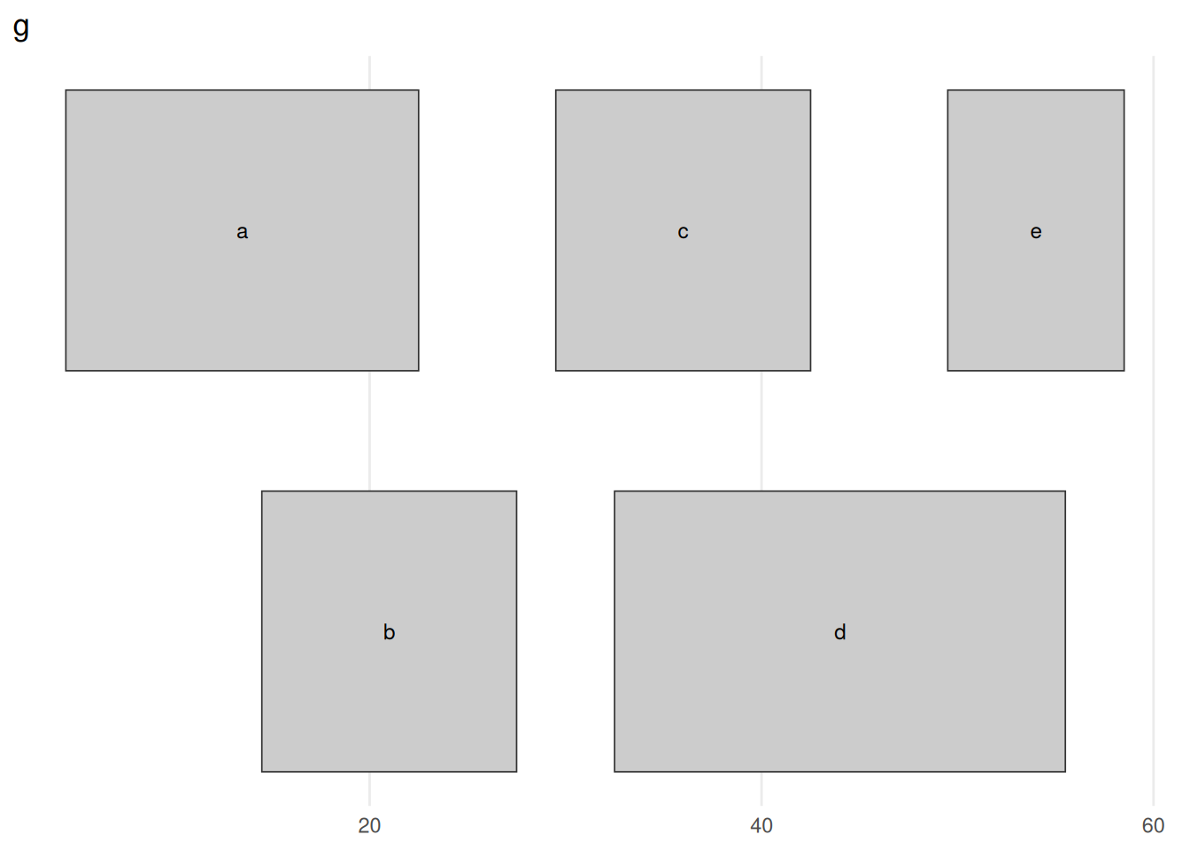

Figure 34.2: Our toy `GRanges` `g`: five ranges on `chr1`, drawn as bars along the coordinate axis. Ranges that would overlap are stacked onto separate rows (`a`, `c`, `e` on top; `b`, `d` below) so each stays visible — the rows carry no meaning beyond avoiding collisions. The ranges form two clusters, `a`/`b` around 5–27 and `c`/`d`/`e` around 30–58, with a clean gap between them at 28–29. Keep this picture in mind: every figure that follows shows what one operation does to it.

The GRanges class has accessors for the “ranges” part of the data. For example:

start(g) # to get start locations

[1]  5 15 30 33 50

end(g)   # to get end locations

[1] 22 27 42 55 58

width(g) # to get the "widths" of each range

[1] 18 13 13 23  9

range(g) # to get the "range" for each sequence (min(start) through max(end))

GRanges object with 1 range and 0 metadata columns:
      seqnames    ranges strand
         <Rle> <IRanges>  <Rle>
  [1]     chr1      5-58      *
  -------
  seqinfo: 1 sequence from an unspecified genome; no seqlengths

The GRanges class has many methods for manipulating ranges, classed as intra-range, inter-range, and between-range methods. Intra-range methods operate on each range independently. The flank() method returns the region flanking each range — the bases immediately upstream (or downstream) of it. This is how you turn a gene into its promoter (the window just upstream of its start), or grab the sequence beside a transcription-factor binding site to scan for a partner’s motif. Which side is “upstream” depends on strand, so to see flank() clearly we switch to a tiny stranded example: one gene p on the + strand and one gene m on the - strand.

gs <- GRanges("chr1",
              IRanges(start = c(10, 40), end = c(25, 55)),
              strand = c("+", "-"))
names(gs) <- c("p", "m")
flank(gs, 8)                # 8 bases upstream of each range

GRanges object with 2 ranges and 0 metadata columns:
    seqnames    ranges strand
       <Rle> <IRanges>  <Rle>
  p     chr1       2-9      +
  m     chr1     56-63      -
  -------
  seqinfo: 1 sequence from an unspecified genome; no seqlengths

flank(gs, 8, start = FALSE) # 8 bases downstream of each range

GRanges object with 2 ranges and 0 metadata columns:
    seqnames    ranges strand
       <Rle> <IRanges>  <Rle>
  p     chr1     26-33      +
  m     chr1     32-39      -
  -------
  seqinfo: 1 sequence from an unspecified genome; no seqlengths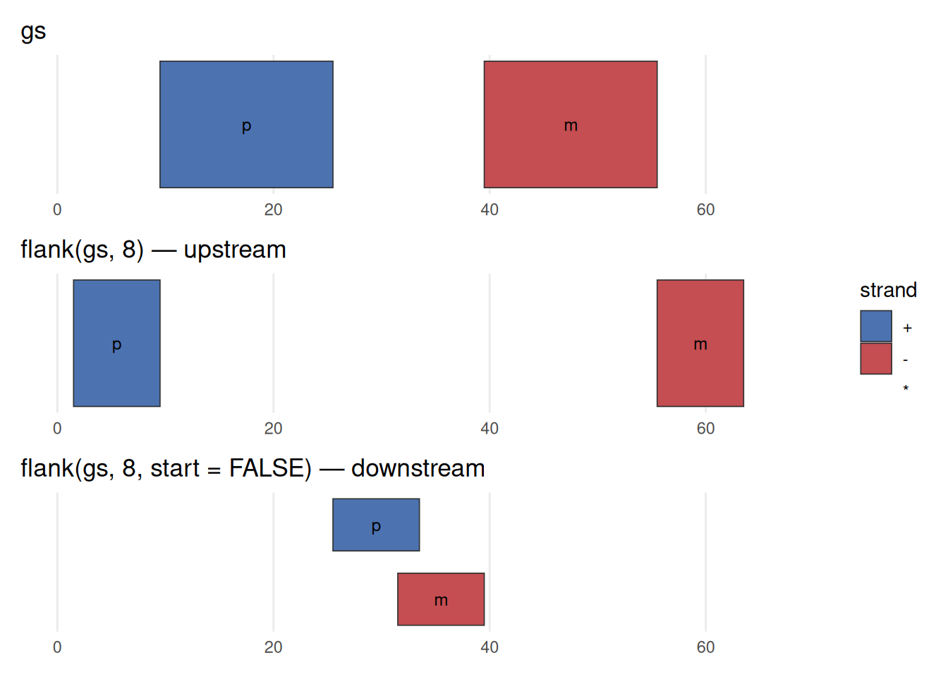

( plot_ranges(gs, "gs", c(0, 68)) /
  plot_ranges(flank(gs, 8), "flank(gs, 8) — upstream", c(0, 68)) /
  plot_ranges(flank(gs, 8, start = FALSE),
              "flank(gs, 8, start = FALSE) — downstream", c(0, 68)) ) +
  plot_layout(guides = "collect")

Figure 34.3: `flank()` is strand-aware. **Top:** the two genes, `p` on the `+` strand (blue) and `m` on the `-` strand (red). **Middle:** `flank(gs, 8)` returns the 8 bases *upstream* of each. For the `+` gene, upstream is to the *left* (lower coordinates); but the `-` gene runs the other way, so its upstream flank sits to the *right* (higher coordinates). **Bottom:** `flank(gs, 8, start = FALSE)` takes the *downstream* side, flipping each flank to the opposite end. The width (8) is the same in every case — only which side, and that side is decided by strand. Forgetting this is a classic source of off-by-a-region bugs.

Strand changes what “upstream” means

For flank(), resize(), precede(), and follow(), “upstream” and “downstream” are interpreted relative to the strand. On the + strand, upstream is toward lower coordinates; on the - strand it is toward higher coordinates. A * (unstranded) range is treated as +. If your ranges have the wrong strand — or you forgot to set it — these operations will silently flank the wrong side. When a result looks backwards, check strand() first.

Two more intra-range methods are shift and resize. shift() slides every range by a fixed number of bases; resize() sets every range to a chosen width. You reach for shift() to apply small systematic coordinate corrections — such as nudging an ATAC-seq fragment end to the Tn5 cut site — and for resize() whenever you need comparable regions: fixed-width windows centred on peak summits for motif discovery, or uniform windows around transcription start sites for a metagene heatmap (exactly what the ATAC-seq chapter builds).

shift(g, 5)

GRanges object with 5 ranges and 1 metadata column:
    seqnames    ranges strand |     score
       <Rle> <IRanges>  <Rle> | <numeric>
  a     chr1     10-27      * |         5
  b     chr1     20-32      * |         8
  c     chr1     35-47      * |         3
  d     chr1     38-60      * |         9
  e     chr1     55-63      * |         6
  -------
  seqinfo: 1 sequence from an unspecified genome; no seqlengths

resize(g, width = 12, fix = "center")

GRanges object with 5 ranges and 1 metadata column:
    seqnames    ranges strand |     score
       <Rle> <IRanges>  <Rle> | <numeric>
  a     chr1      8-19      * |         5
  b     chr1     15-26      * |         8
  c     chr1     30-41      * |         3
  d     chr1     38-49      * |         9
  e     chr1     48-59      * |         6
  -------
  seqinfo: 1 sequence from an unspecified genome; no seqlengths

before_after(g, shift(g, 5), "shift(g, 5)")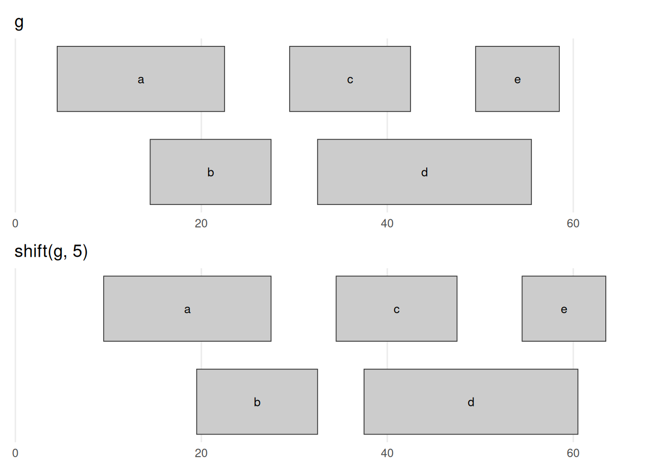

Figure 34.4: `shift(g, 5)` slides every range 5 bases toward higher coordinates — the entire picture moves right by 5, and nothing else changes. Every width is preserved and the overlaps are carried along unchanged; only position moves. A negative number shifts left.

before_after(g, resize(g, width = 12, fix = "center"),
             'resize(g, width = 12, fix = "center")')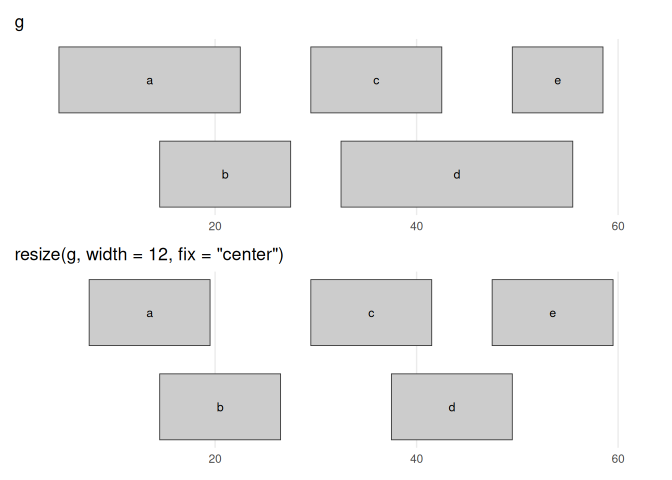

Figure 34.5: `resize(g, width = 12, fix = "center")` forces every range to width 12, holding each range’s *centre* fixed so it grows or shrinks symmetrically: the wide ranges (`a`, `d`) contract and the narrow one (`e`) expands, until all are equal width. The `fix` argument chooses the anchor — `fix = "start"` or `"end"` instead pin one end in place, and, exactly as with `flank()`, *which* physical end that is depends on strand (these ranges are unstranded, so `"start"` means the lower coordinate).

The GenomicRanges help page ?"intra-range-methods" summarizes these methods.

34.2.2.2 Inter-range methods

Inter-range methods involve comparisons between ranges in a single GRanges object. For instance, the reduce method will align the ranges and merge overlapping ranges to produce a simplified set.

reduce(g)

GRanges object with 2 ranges and 0 metadata columns:
      seqnames    ranges strand
         <Rle> <IRanges>  <Rle>
  [1]     chr1      5-27      *
  [2]     chr1     30-58      *
  -------
  seqinfo: 1 sequence from an unspecified genome; no seqlengths

before_after(g, reduce(g), "reduce(g)")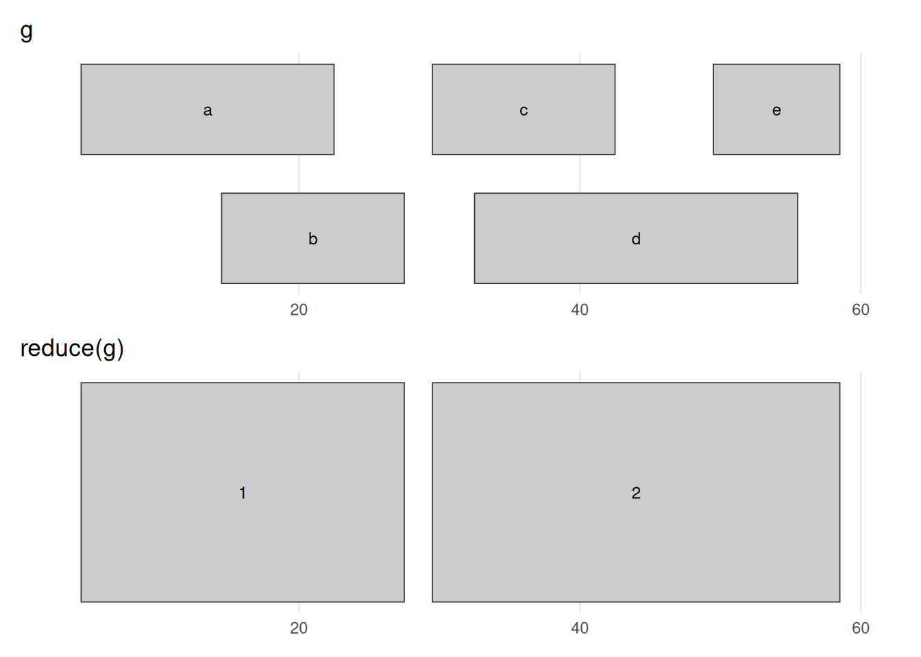

Figure 34.6: `reduce(g)` merges every group of overlapping or touching ranges into the smallest set that covers exactly the same bases. The five input ranges collapse to two: the `a`/`b` overlap becomes 5–27 and the `c`/`d`/`e` overlap becomes 30–58. The 28–29 gap survives, because no input range covered those bases. This is the standard way to turn a pile of overlapping annotations (say, exons from many transcripts) into one non-redundant set of covered regions.

For example, a gene’s exons — pooled across all of its transcripts — overlap heavily; reduce() collapses them into the gene’s non-redundant exonic footprint, the set you would sum to answer “how many bases of this gene are exonic?”. The same move merges peak calls from several replicates into one consensus set.

Sometimes you care about what lies between the ranges. If the ranges are a gene’s exons, the gaps between them are its introns; if they are all the genes on a chromosome, the gaps are the intergenic regions. The gaps method provides them:

gaps(g)

GRanges object with 2 ranges and 0 metadata columns:
      seqnames    ranges strand
         <Rle> <IRanges>  <Rle>
  [1]     chr1       1-4      *
  [2]     chr1     28-29      *
  -------
  seqinfo: 1 sequence from an unspecified genome; no seqlengths

before_after(g, gaps(g), "gaps(g)")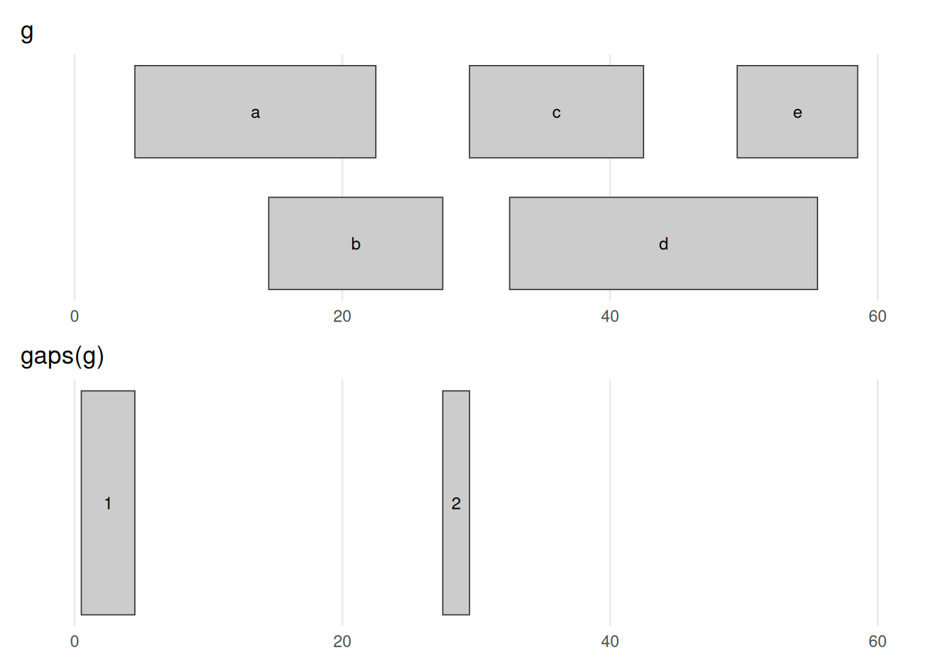

Figure 34.7: `gaps(g)` returns the complement of `g` — the stretches *not* covered by any range. The informative one is 28–29, the gap between the two clusters; the 1–4 stretch before the first range also appears. (The gap *after* the last range is missing because the object has no chromosome length to mark where `chr1` ends — see the warning below.) `gaps()` and `reduce()` are mirror images: one returns what is covered, the other what is not.

gaps() needs to know how long each chromosome is

We never told this object how long the chromosomes are, so Bioconductor assumes each chromosome ends at the largest coordinate it has seen. That means the final gap (from the last range to the true end of the chromosome) is missing. In real work you set the chromosome lengths with seqlengths() so that gaps(), coverage(), and friends know the full extent of each sequence. We can ignore that detail for these toy examples.

The disjoin method represents a GRanges object as a collection of non-overlapping ranges. This is the step before counting: once a region is split into pieces that each belong to a fixed set of features, a read landing in a piece can be attributed to those features unambiguously.

disjoin(g)

GRanges object with 8 ranges and 0 metadata columns:
      seqnames    ranges strand
         <Rle> <IRanges>  <Rle>
  [1]     chr1      5-14      *
  [2]     chr1     15-22      *
  [3]     chr1     23-27      *
  [4]     chr1     30-32      *
  [5]     chr1     33-42      *
  [6]     chr1     43-49      *
  [7]     chr1     50-55      *
  [8]     chr1     56-58      *
  -------
  seqinfo: 1 sequence from an unspecified genome; no seqlengths

before_after(g, disjoin(g), "disjoin(g)")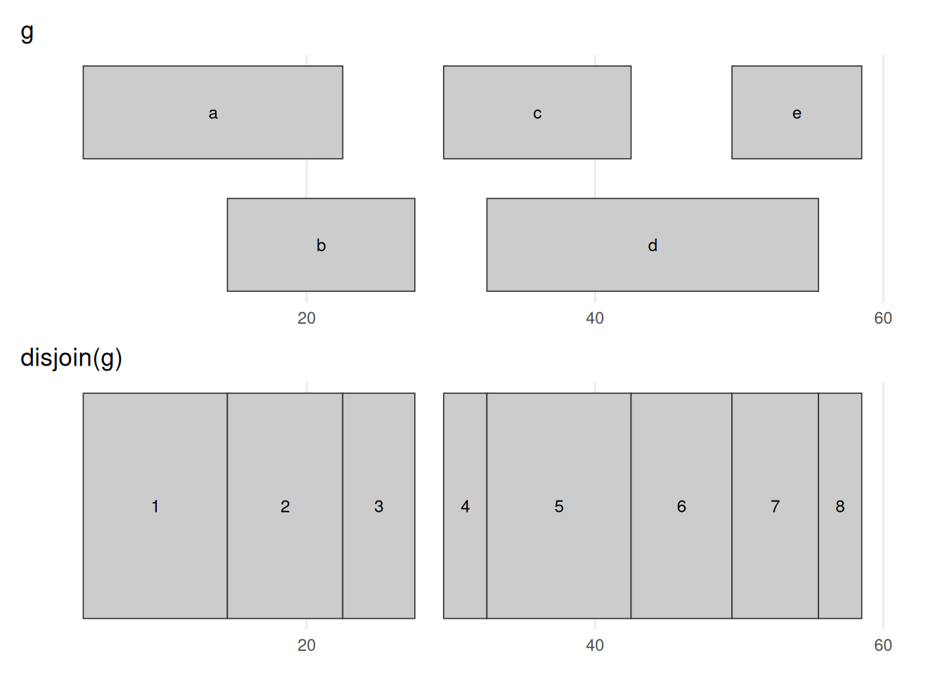

Figure 34.8: `disjoin(g)` cuts the ranges at every start and end into non-overlapping pieces, so that within each output piece the *same* set of input ranges is present throughout. Where ranges overlapped — `b` over `a`, or `d` over `c` and `e` — the region is carved into separate before / overlap / after segments, giving eight pieces here. Unlike `reduce()`, which merges, `disjoin()` subdivides; it is the machinery behind per-base summaries such as coverage, computed next.

The coverage method counts, base by base, how many ranges overlap each position — and it is the workhorse of sequencing analysis. Pile up aligned reads and the tall stacks are where signal concentrates: the peaks of a ChIP-seq or ATAC-seq experiment, or the per-exon read depth behind an RNA-seq count.

coverage(g)

RleList of length 1
$chr1
integer-Rle of length 58 with 10 runs
  Lengths:  4 10  8  5  2  3 10  7  6  3
  Values :  0  1  2  1  0  1  2  1  2  1

The coverage is summarized as a list of coverages, one for each chromosome. The Rle class is used to store the values. Sometimes, one must convert these values to numeric using as.numeric. In many cases, this will happen automatically, though.

xl <- c(0, 62)
(plot_ranges(g, "g", xl) / plot_coverage(g, xl)) + plot_layout(heights = c(2, 1))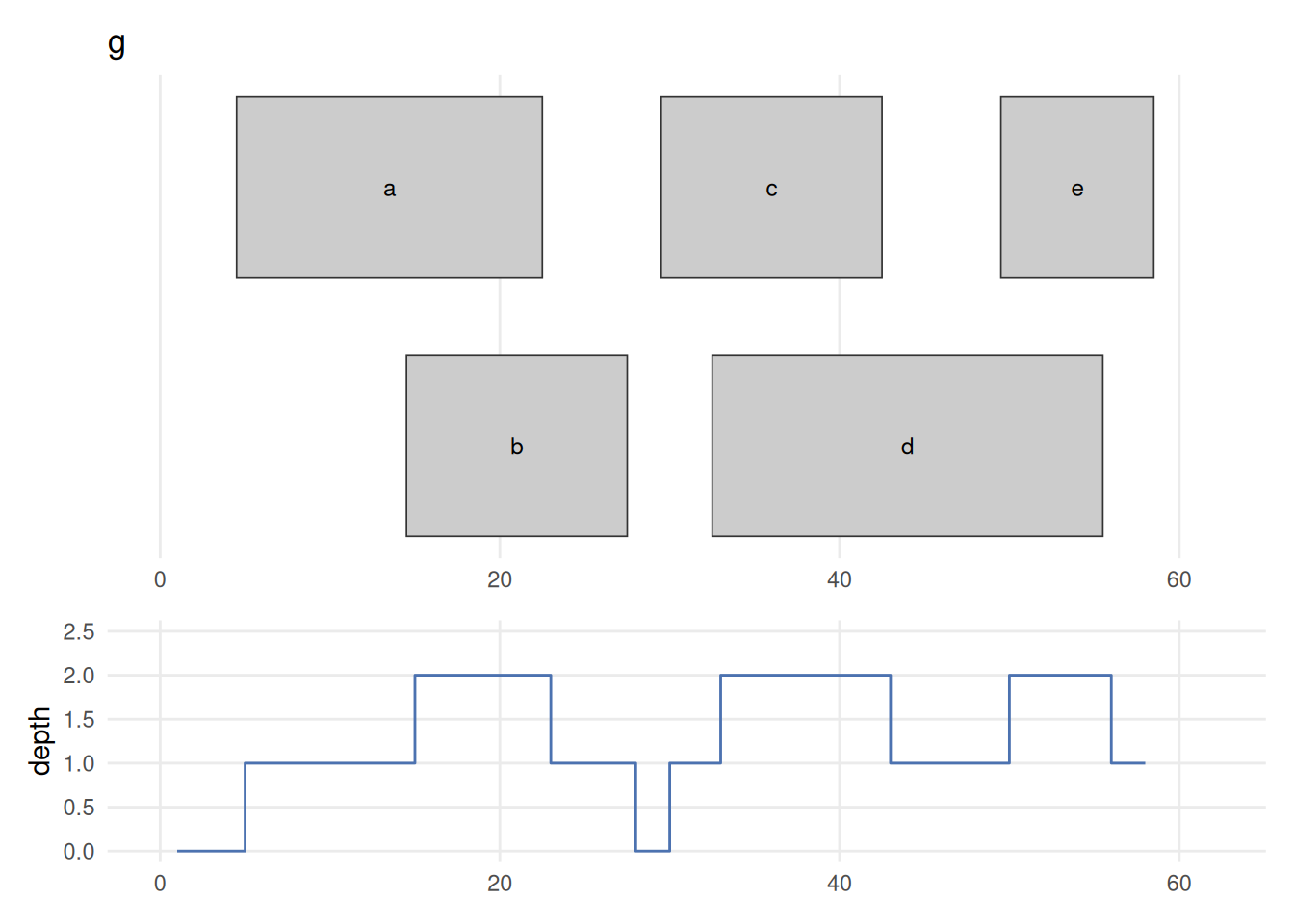

Figure 34.9: `coverage(g)` counts, at every base, how many ranges overlap that position. Drawing the ranges (top) directly above their coverage (bottom) makes the link plain: depth is 1 under a lone range, steps up to 2 wherever two ranges overlap (the `a`/`b` overlap, and the `c`/`d` and `d`/`e` overlaps), and drops to 0 across the 28–29 gap. This is the per-base signal you compute from piled-up sequencing reads — the tall stacks are the peaks a ChIP-seq or ATAC-seq experiment hunts for.

See the GenomicRanges help page ?"intra-range-methods" for more details.

34.2.3 Set operations for GRanges objects

Between-range methods calculate relationships between different GRanges objects. Of central importance are findOverlaps and related operations; these are discussed below. Additional operations treat GRanges as mathematical sets of coordinates; union(g, g2) is the union of the coordinates in g and g2. Here we compare g with a second set g2 (also on chr1, overlapping g in places), calculating the union, the intersection, and the asymmetric difference (setdiff). These are everyday tools for comparing experiments: intersect() two replicate peak sets to keep the peaks they agree on, setdiff() to find condition-specific peaks, or intersect peaks with promoters to count how many binding sites fall in a promoter.

g2 <- GRanges("chr1", IRanges(c(24, 62), c(36, 70)))
names(g2) <- c("x", "y")
GenomicRanges::union(g, g2)

GRanges object with 2 ranges and 0 metadata columns:
      seqnames    ranges strand
         <Rle> <IRanges>  <Rle>
  [1]     chr1      5-58      *
  [2]     chr1     62-70      *
  -------
  seqinfo: 1 sequence from an unspecified genome; no seqlengths

GenomicRanges::intersect(g, g2)

GRanges object with 2 ranges and 0 metadata columns:
      seqnames    ranges strand
         <Rle> <IRanges>  <Rle>
  [1]     chr1     24-27      *
  [2]     chr1     30-36      *
  -------
  seqinfo: 1 sequence from an unspecified genome; no seqlengths

GenomicRanges::setdiff(g, g2)

GRanges object with 2 ranges and 0 metadata columns:
      seqnames    ranges strand
         <Rle> <IRanges>  <Rle>
  [1]     chr1      5-23      *
  [2]     chr1     37-58      *
  -------
  seqinfo: 1 sequence from an unspecified genome; no seqlengths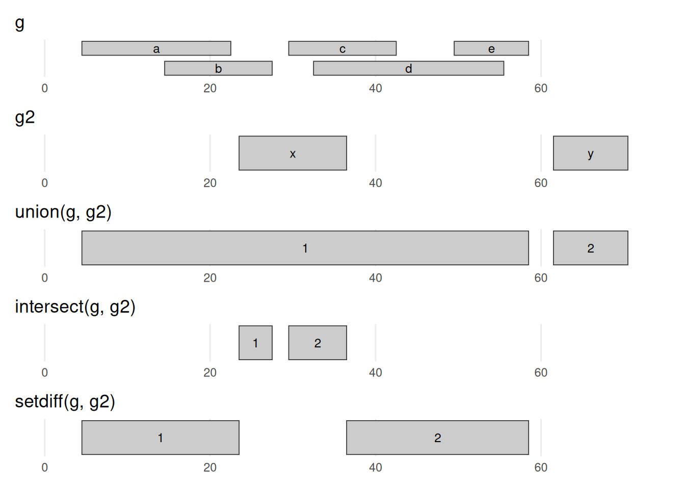

Figure 34.10: The three set operations on `g` and `g2`, drawn on a shared axis. **union** keeps every base in *either* set — here `g2`’s range `x` bridges `g`’s two clusters into one 5–58 range, while `y` stays separate. **intersect** keeps only bases in *both* sets (the slivers where `x` overlaps `b`/`c`/`d`). **setdiff(g, g2)** keeps the bases of `g` that are *not* in `g2` (it carves `x`’s footprint out of `g`). Read against the `g`/`g2` rows at the top, this is the coordinate bookkeeping behind comparing two experiments — shared peaks, or peaks unique to one condition.

There is extensive additional help in the vignettes at the GenomicRanges pages.

?GRanges

There are also many possible methods that work with GRanges objects. To see a complete list (long), try:

methods(class="GRanges")

34.3 GRangesList

Some important genomic features, such as spliced transcripts that are comprised of exons, are inherently compound structures. Such a feature makes much more sense when expressed as a compound object such as a GRangesList. If we think of each transcript as a set of exons, each transcript would be summarized as a GRanges object. However, if we have multiple transcripts, we want to keep them separate, with each transcript holding its own exons. A GRangesList is a list of GRanges objects. Continuing with the transcripts idea, a GRangesList can contain all the transcripts and their exons; each transcript is one element in the list.

Figure 34.11: The structure of a GRangesList, which is a `list` of GRanges objects. While the analogy is not perfect, a `GRangesList` behaves a bit like a list. Each element in the `GRangesList` is a `GRanges` object. A common use case for a `GRangesList` is to store a list of transcripts, each of which have exons as the regions in the `GRanges`.

Whenever genomic features consist of multiple ranges that are grouped by a parent feature, they can be represented as a GRangesList object. Consider the simple example of the two transcript GRangesList below created using the GRangesList constructor.

gr1 <- GRanges(
    seqnames = "chr1", 
    ranges = IRanges(103, 106),
    strand = "+", 
    score = 5L, GC = 0.45)
gr2 <- GRanges(
    seqnames = c("chr1", "chr1"),
    ranges = IRanges(c(107, 113), width = 3),
    strand = c("+", "-"), 
    score = 3:4, GC = c(0.3, 0.5))

The gr1 and gr2 are each GRanges objects. We can combine them into a “named” GRangesList like so:

grl <- GRangesList("txA" = gr1, "txB" = gr2)
grl

GRangesList object of length 2:
$txA
GRanges object with 1 range and 2 metadata columns:
      seqnames    ranges strand |     score        GC
         <Rle> <IRanges>  <Rle> | <integer> <numeric>
  [1]     chr1   103-106      + |         5      0.45
  -------
  seqinfo: 1 sequence from an unspecified genome; no seqlengths

$txB
GRanges object with 2 ranges and 2 metadata columns:
      seqnames    ranges strand |     score        GC
         <Rle> <IRanges>  <Rle> | <integer> <numeric>
  [1]     chr1   107-109      + |         3       0.3
  [2]     chr1   113-115      - |         4       0.5
  -------
  seqinfo: 1 sequence from an unspecified genome; no seqlengths

The show method for a GRangesList object displays it as a named list of GRanges objects, where the names of this list are considered to be the names of the grouping feature. In the example above, the groups of individual exon ranges are represented as separate GRanges objects which are further organized into a list structure where each element name is a transcript name. Many other combinations of grouped and labeled GRanges objects are possible of course, but this example is a common arrangement.

In some cases, GRangesLists behave quite similarly to GRanges objects.

34.3.1 Basic GRangesList accessors

Just as with GRanges object, the components of the genomic coordinates within a GRangesList object can be extracted using simple accessor methods. Not surprisingly, the GRangesList objects have many of the same accessors as GRanges objects. The difference is that many of these methods return a list since the input is now essentially a list of GRanges objects. Here are a few examples:

seqnames(grl)

RleList of length 2
$txA
factor-Rle of length 1 with 1 run
  Lengths:    1
  Values : chr1
Levels(1): chr1

$txB
factor-Rle of length 2 with 1 run
  Lengths:    2
  Values : chr1
Levels(1): chr1

ranges(grl)

IRangesList object of length 2:
$txA
IRanges object with 1 range and 0 metadata columns:
          start       end     width
      <integer> <integer> <integer>
  [1]       103       106         4

$txB
IRanges object with 2 ranges and 0 metadata columns:
          start       end     width
      <integer> <integer> <integer>
  [1]       107       109         3
  [2]       113       115         3

strand(grl)

RleList of length 2
$txA
factor-Rle of length 1 with 1 run
  Lengths: 1
  Values : +
Levels(3): + - *

$txB
factor-Rle of length 2 with 2 runs
  Lengths: 1 1
  Values : + -
Levels(3): + - *

The length and names methods will return the length or names of the list and the seqlengths method will return the set of sequence lengths.

length(grl)

[1] 2

names(grl)

[1] "txA" "txB"

seqlengths(grl)

chr1 
  NA

34.4 Relationships between region sets

One of the more powerful approaches to genomic data integration is to ask about the relationship between sets of genomic ranges. The key features of this process are to look at overlaps and distances to the nearest feature. These functionalities, combined with the operations like flank and resize, for instance, allow pretty useful analyses with relatively little code. In general, these operations are very fast, even on thousands to millions of regions.

34.4.1 Overlaps

The findOverlaps method in the GenomicRanges package is a very useful function that allows users to identify overlaps between two sets of genomic ranges.

Here’s how it works:

Inputs

The function requires two GRanges objects, referred to as query and subject.
Processing

The function then compares every range in the query object with every range in the subject object, looking for overlaps. An overlap is defined as any instance where the range in the query object intersects with a range in the subject object.
Output

The function returns a Hits (see ?Hits) object, which is a compact representation of the matrix of overlaps. Each entry in the Hits object corresponds to a pair of overlapping ranges, with the query index and the subject index.

Here is an example, reusing g as the query and g2 as the subject:

overlaps <- findOverlaps(query = g, subject = g2)
overlaps

Hits object with 3 hits and 0 metadata columns:
      queryHits subjectHits
      <integer>   <integer>
  [1]         2           1
  [2]         3           1
  [3]         4           1
  -------
  queryLength: 5 / subjectLength: 2

Each row of the Hits object is an overlapping pair: the first column is the index of the range in g, the second the index of the overlapping range in g2. Ranges b, c, and d of g all overlap g2’s first range (x), while g2’s second range (y) is hit by nothing — Figure 34.12 shows exactly this.

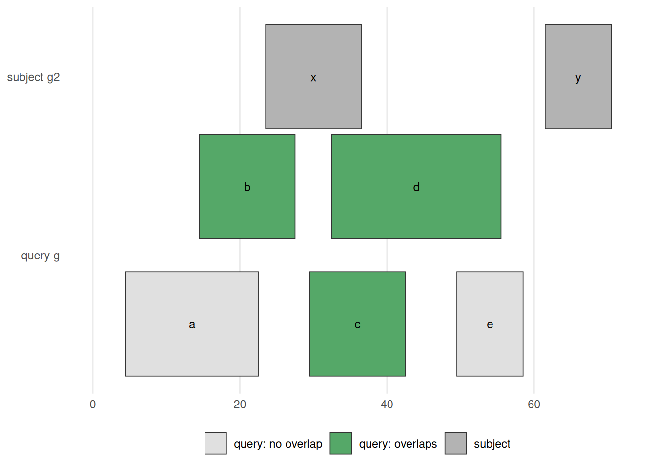
Figure 34.12: `findOverlaps(g, g2)` / `g %over% g2`. The subject `g2` is drawn on top; the query `g` below, with each range coloured green if it overlaps the subject and grey if not. Ranges `b`, `c`, `d` overlap `g2`‘s range `x` and so are green; `a` and `e` touch nothing and stay grey; `g2`’s range `y` has no query over it. This is the picture behind every overlap question — ’which peaks fall in a promoter?’, ‘which variants land in an exon?’

If you want only the queryHits or the subjectHits, there are accessors for those (e.g. queryHits(overlaps)). Used as an index into the original objects, they pull out the ranges that overlap:

g[queryHits(overlaps)]

GRanges object with 3 ranges and 1 metadata column:
    seqnames    ranges strand |     score
       <Rle> <IRanges>  <Rle> | <numeric>
  b     chr1     15-27      * |         8
  c     chr1     30-42      * |         3
  d     chr1     33-55      * |         9
  -------
  seqinfo: 1 sequence from an unspecified genome; no seqlengths

g2[subjectHits(overlaps)]

GRanges object with 3 ranges and 0 metadata columns:
    seqnames    ranges strand
       <Rle> <IRanges>  <Rle>
  x     chr1     24-36      *
  x     chr1     24-36      *
  x     chr1     24-36      *
  -------
  seqinfo: 1 sequence from an unspecified genome; no seqlengths

As you might expect, the countOverlaps method counts, for each range in the first GRanges, how many ranges in the second it overlaps.

countOverlaps(g, g2)

a b c d e 
0 1 1 1 0

The subsetByOverlaps method simply subsets the query GRanges object to include only those that overlap the subject — the green ranges in Figure 34.12.

subsetByOverlaps(g, g2)

GRanges object with 3 ranges and 1 metadata column:
    seqnames    ranges strand |     score
       <Rle> <IRanges>  <Rle> | <numeric>
  b     chr1     15-27      * |         8
  c     chr1     30-42      * |         3
  d     chr1     33-55      * |         9
  -------
  seqinfo: 1 sequence from an unspecified genome; no seqlengths

In some cases, you may want only one hit per query range. The select parameter handles this: with select="first", findOverlaps() returns a plain integer vector with one entry per query range (the index of its first overlapping subject, or NA if there is none) instead of a full Hits object.

findOverlaps(g, g2, select="first")

[1] NA  1  1  1 NA

The %over% logical operator is the quick version: it returns TRUE/FALSE for each query range, which is handy for subsetting.

g %over% g2

[1] FALSE  TRUE  TRUE  TRUE FALSE

g[g %over% g2]

GRanges object with 3 ranges and 1 metadata column:
    seqnames    ranges strand |     score
       <Rle> <IRanges>  <Rle> | <numeric>
  b     chr1     15-27      * |         8
  c     chr1     30-42      * |         3
  d     chr1     33-55      * |         9
  -------
  seqinfo: 1 sequence from an unspecified genome; no seqlengths

34.4.2 Nearest feature

There are a number of useful methods that find the nearest feature in a second set for each element in the first — answering a question you meet constantly: which gene is this peak closest to? Annotating each ChIP-seq peak with its nearest transcription start site, or reporting how far a variant sits from the nearest gene, is a single nearest() or distanceToNearest() call.

We can review the two GRanges toy objects we’ll compare — g and the second set g2 from the set-operations section:

GRanges object with 5 ranges and 1 metadata column:
    seqnames    ranges strand |     score
       <Rle> <IRanges>  <Rle> | <numeric>
  a     chr1      5-22      * |         5
  b     chr1     15-27      * |         8
  c     chr1     30-42      * |         3
  d     chr1     33-55      * |         9
  e     chr1     50-58      * |         6
  -------
  seqinfo: 1 sequence from an unspecified genome; no seqlengths

g2

GRanges object with 2 ranges and 0 metadata columns:
    seqnames    ranges strand
       <Rle> <IRanges>  <Rle>
  x     chr1     24-36      *
  y     chr1     62-70      *
  -------
  seqinfo: 1 sequence from an unspecified genome; no seqlengths

nearest: Performs conventional nearest neighbor finding. Returns an integer vector containing the index of the nearest neighbor range in subject for each range in x. If there is no nearest neighbor NA is returned. For details of the algorithm see the man page in the IRanges package (?nearest).
precede: For each range in x, precede returns the index of the range in subject that is directly preceded by the range in x. Overlapping ranges are excluded. NA is returned when there are no qualifying ranges in subject.
follow: The opposite of precede, follow returns the index of the range in subject that is directly followed by the range in x. Overlapping ranges are excluded. NA is returned when there are no qualifying ranges in subject.

Orientation and strand for precede and follow: Orientation is 5’ to 3’, consistent with the direction of translation. Because positional numbering along a chromosome is from left to right and transcription takes place from 5’ to 3’, precede and follow can appear to have ‘opposite’ behavior on the + and - strand. Using positions 5 and 6 as an example, 5 precedes 6 on the + strand but follows 6 on the - strand.

The table below outlines the orientation when ranges on different strands are compared. In general, a feature on * is considered to belong to both strands. The single exception is when both x and subject are * in which case both are treated as +.

       x  |  subject  |  orientation 
     -----+-----------+----------------
a)     +  |  +        |  ---> 
b)     +  |  -        |  NA
c)     +  |  *        |  --->
d)     -  |  +        |  NA
e)     -  |  -        |  <---
f)     -  |  *        |  <---
g)     *  |  +        |  --->
h)     *  |  -        |  <---
i)     *  |  *        |  --->  (the only situation where * arbitrarily means +)

res <- nearest(g, g2)
res

[1] 1 1 1 1 2

Each element of res is the index into g2 of the nearest range to the corresponding range in g. So g2[res] would give you the actual nearest ranges.

While nearest and friends give the index of the nearest feature, the distance to the nearest is sometimes also useful to have. The distanceToNearest method calculates the nearest feature as well as reporting the distance.

res <- distanceToNearest(g, g2)
res

Hits object with 5 hits and 1 metadata column:
      queryHits subjectHits |  distance
      <integer>   <integer> | <integer>
  [1]         1           1 |         1
  [2]         2           1 |         0
  [3]         3           1 |         0
  [4]         4           1 |         0
  [5]         5           2 |         3
  -------
  queryLength: 5 / subjectLength: 2

This returns a Hits object with an extra distance column. Several of g’s ranges overlap g2 and so report distance 0; the rest report the gap in base pairs to their nearest neighbour (range a is 1 bp from g2’s first range, and e is 3 bp from its second).

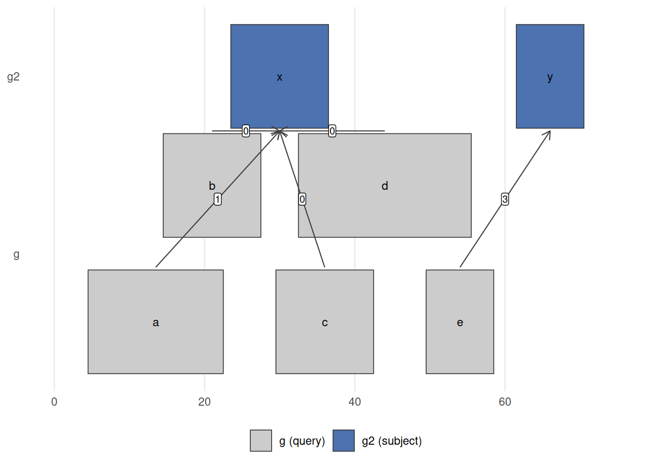
Figure 34.13: `nearest(g, g2)` links each query range in `g` (bottom) to its closest range in `g2` (top); the label on each arrow is the `distanceToNearest()` distance. Ranges `b`, `c`, `d` sit on top of `g2`‘s range `x`, so their distance is 0; `a` is 1 bp away and `e` is 3 bp from `g2`’s range `y`. This is the operation behind ’assign each ChIP-seq peak to its nearest gene’ or ‘how far is this variant from the closest transcription start site?’

34.5 Gene models

So far every range has been one we typed by hand. In practice you usually pull ranges from an annotation. A TxDb (“transcript database”) package provides a convenient interface to gene models from a variety of sources. The TxDb.Hsapiens.UCSC.hg38.knownGene package provides access to the UCSC knownGene gene model for the hg38 build of the human genome. Everything it returns is a GRanges (or GRangesList), so all the operations from this chapter apply directly.

Figure 34.14: A graphical representation of range operations demonstrated on a gene model.

# install once: BiocManager::install("TxDb.Hsapiens.UCSC.hg38.knownGene")
library(TxDb.Hsapiens.UCSC.hg38.knownGene)
txdb <- TxDb.Hsapiens.UCSC.hg38.knownGene

The transcripts function returns a GRanges object with the transcripts for all genes in the database.

tx <- transcripts(txdb)
tx

GRanges object with 412044 ranges and 2 metadata columns:
                      seqnames        ranges strand |     tx_id
                         <Rle>     <IRanges>  <Rle> | <integer>
       [1]                chr1   11121-14413      + |         1
       [2]                chr1   11125-14405      + |         2
       [3]                chr1   11410-14413      + |         3
       [4]                chr1   11411-14413      + |         4
       [5]                chr1   11426-14409      + |         5
       ...                 ...           ...    ... .       ...
  [412040] chrX_MU273397v1_alt 239036-260095      - |    412040
  [412041] chrX_MU273397v1_alt 272358-282686      - |    412041
  [412042] chrX_MU273397v1_alt 314193-316302      - |    412042
  [412043] chrX_MU273397v1_alt 314813-315236      - |    412043
  [412044] chrX_MU273397v1_alt 324527-324923      - |    412044
                     tx_name
                 <character>
       [1] ENST00000832824.1
       [2] ENST00000832825.1
       [3] ENST00000832826.1
       [4] ENST00000832827.1
       [5] ENST00000832828.1
       ...               ...
  [412040] ENST00000710260.1
  [412041] ENST00000710028.1
  [412042] ENST00000710030.1
  [412043] ENST00000710216.1
  [412044] ENST00000710031.1
  -------
  seqinfo: 711 sequences (1 circular) from hg38 genome

The exons function returns a GRanges object with the exons.

ex <- exons(txdb)
ex

GRanges object with 966596 ranges and 1 metadata column:
                      seqnames        ranges strand |   exon_id
                         <Rle>     <IRanges>  <Rle> | <integer>
       [1]                chr1   11121-11211      + |         1
       [2]                chr1   11125-11211      + |         2
       [3]                chr1   11410-11671      + |         3
       [4]                chr1   11411-11671      + |         4
       [5]                chr1   11426-11671      + |         5
       ...                 ...           ...    ... .       ...
  [966592] chrX_MU273397v1_alt 314193-314248      - |    966592
  [966593] chrX_MU273397v1_alt 314813-315236      - |    966593
  [966594] chrX_MU273397v1_alt 315258-315407      - |    966594
  [966595] chrX_MU273397v1_alt 316254-316302      - |    966595
  [966596] chrX_MU273397v1_alt 324527-324923      - |    966596
  -------
  seqinfo: 711 sequences (1 circular) from hg38 genome

The genes function returns a GRanges object with one range per gene.

gn <- genes(txdb)
gn

GRanges object with 35356 ranges and 1 metadata column:
            seqnames              ranges strand |     gene_id
               <Rle>           <IRanges>  <Rle> | <character>
          1    chr19   58345178-58362751      - |           1
         10     chr8   18386273-18401218      + |          10
        100    chr20   44584896-44652252      - |         100
       1000    chr18   27932879-28177946      - |        1000
  100008586     chrX   49551278-49568218      + |   100008586
        ...      ...                 ...    ... .         ...
       9990    chr15   34229784-34338060      - |        9990
       9991     chr9 112215071-112333653      - |        9991
       9992    chr21   34180729-34371381      + |        9992
       9993    chr22   19036282-19122454      - |        9993
       9997    chr22   50523568-50526461      - |        9997
  -------
  seqinfo: 711 sequences (1 circular) from hg38 genome

Notice the scale: these are real GRanges objects with tens of thousands of ranges, yet they print and subset instantly. That is the payoff of the compact representation — the same findOverlaps(), nearest(), and subsetByOverlaps() calls you practiced on the toy gr work unchanged here. For example, subsetByOverlaps(gn, peaks) would give you the genes hit by a set of ChIP-seq peaks, and nearest(peaks, tx) would assign each peak to its closest transcript.

Grouping exons by transcript

exons(txdb) gives you a flat GRanges of every exon. When you instead want the exons grouped by the transcript they belong to — a GRangesList, one element per transcript — use exonsBy(txdb, by = "tx"). That is the natural object for counting reads per transcript and is exactly the GRangesList structure we built by hand earlier.

34.6 Quick reference: GRanges methods

Every method below was introduced by example earlier in the chapter; this is a compact place to look them back up. Figure 34.15 shows the single-set reshaping operations side by side.

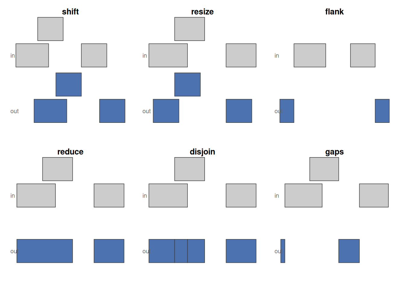
Figure 34.15: The single-set range operations at a glance: in each panel the grey ranges are the input and the blue ranges are the result. `shift` slides, `resize` standardises width, `flank` takes the region beside each range (strand-aware, so the two strands flank opposite ends), `reduce` merges overlaps, `disjoin` cuts into non-overlapping pieces, and `gaps` returns what is left uncovered.

Accessors pull pieces out of a GRanges:

Accessor	Returns
`length`	Number of ranges in the object
`seqnames`	Chromosome of each range
`ranges`, `start`, `end`, `width`	The coordinates, and the widths
`strand`	Strand (`+`, `-`, or `*`) of each range
`mcols` (a.k.a. `elementMetadata`)	The metadata columns (right of the `\|`)
`seqlevels`, `seqinfo`	Sequence names, and names + lengths
`[`, `subset`, `sort`	Subset, filter, or sort the ranges

Table 34.2: Accessors for a GRanges.

Operations transform or relate ranges. They fall into three families: those that reshape each range on its own (intra-range), those that summarize a set together (inter-range), and those that relate two sets (between-set).

Operation	Family	What it does	Biological example
`shift`	intra-range	Slide each range by a fixed offset	Apply the Tn5 +4/-5 shift to ATAC-seq reads
`resize`	intra-range	Set each range to a fixed width (anchor with `fix`)	Fixed-width windows on peak summits for motif scanning
`flank`	intra-range	Region beside each range (strand-aware)	Take the promoter just upstream of a gene
`reduce`	inter-range	Merge overlapping or adjacent ranges	Collapse a gene’s exons into its exonic footprint; merge replicate peaks
`disjoin`	inter-range	Cut into non-overlapping pieces	Partition a locus so each read counts once
`gaps`	inter-range	The bases not covered	Introns from exons; intergenic regions from genes
`coverage`	inter-range	Per-base count of overlapping ranges	Pile reads into ChIP-seq/ATAC peaks; per-exon RNA-seq depth
`findOverlaps`, `%over%`	between-set	Which query ranges hit which subject ranges	Which peaks fall in a promoter?
`countOverlaps`	between-set	How many subject ranges each query hits	Count reads per gene
`subsetByOverlaps`	between-set	Keep query ranges overlapping the subject	Keep variants inside exons
`nearest`, `distanceToNearest`	between-set	Closest subject range to each query (+ distance)	Annotate each peak with its nearest gene/TSS
`union`, `intersect`, `setdiff`	between-set	Set arithmetic on two range sets	Reproducible peaks (`intersect`); condition-specific peaks (`setdiff`)

Table 34.3: Range operations, by family, with a biological use for each.

34.7 Summary

You now have a working vocabulary for genomic locations.

A GRanges object holds a set of ranges. Coordinates (seqnames, ranges, strand) sit to the left of the |; optional metadata reached with mcols() sits to the right. You can build one from scratch or coerce a data.frame with as(df, "GRanges").
Intra-range operations (flank(), shift(), resize()) reshape each range on its own and respect strand. Inter-range operations (reduce(), disjoin(), gaps(), coverage()) summarize a set of ranges together.
Between-set operations answer the integration questions: findOverlaps() and subsetByOverlaps() for overlap, nearest() and distanceToNearest() for proximity, plus union()/intersect()/setdiff() for set arithmetic.
A GRangesList groups ranges by a parent feature, such as exons within a transcript.
A TxDb package (here TxDb.Hsapiens.UCSC.hg38.knownGene) hands you real gene, transcript, and exon models as GRanges, so every operation above applies to genome-scale annotation with no new syntax.

Next, the Genomic ranges with real ChIP-seq peaks chapter puts these tools to work on a real peak set imported from file, and the Ranges Exercises then turn you loose on published ENCODE data.

34.8 Exercises

These reuse the objects built earlier in the chapter: the 10-range gr, the small single-chromosome toy g and its companion g2, and the grl GRangesList. Run the chapter’s chunks first so those objects exist.

1. Read the structure. Without running any code, which of these belong to the left of the | in a GRanges (the coordinates) and which to the right (the metadata): strand, score, seqnames, GC, width?

Solution

Left of the | (coordinates): seqnames, strand, and width (part of ranges). Right of the | (metadata): score and GC. The coordinate columns have dedicated accessors; the metadata columns are reached together with mcols().

2. Promoters by hand. A common task is to grab the region just upstream of a feature’s start — a rough promoter. Use flank() to get the 50 bases upstream of each range in g, then confirm with width() that each result is 50 bases wide.

Solution

prom <- flank(g, 50)
prom

GRanges object with 5 ranges and 1 metadata column:
    seqnames    ranges strand |     score
       <Rle> <IRanges>  <Rle> | <numeric>
  a     chr1     -45-4      * |         5
  b     chr1    -35-14      * |         8
  c     chr1    -20-29      * |         3
  d     chr1    -17-32      * |         9
  e     chr1      0-49      * |         6
  -------
  seqinfo: 1 sequence from an unspecified genome; no seqlengths

width(prom)

[1] 50 50 50 50 50

flank() defaults to the upstream side (start = TRUE), measured relative to strand. Every flank is exactly 50 bases wide.

3. Collapse overlaps. Use reduce() on gr to merge overlapping or adjacent ranges into a minimal set, then report how many ranges remain with length().

Solution

reduced <- reduce(gr)
reduced

GRanges object with 7 ranges and 0 metadata columns:
      seqnames    ranges strand
         <Rle> <IRanges>  <Rle>
  [1]     chr1   106-116      +
  [2]     chr1   101-111      -
  [3]     chr1   105-115      *
  [4]     chr2   102-113      +
  [5]     chr2   104-114      *
  [6]     chr3   107-118      +
  [7]     chr3   109-120      -
  -------
  seqinfo: 3 sequences from an unspecified genome; no seqlengths

length(reduced)

[1] 7

reduce() works per chromosome and per strand, merging ranges that overlap or abut into single ranges — the standard way to collapse overlapping exons into non-redundant regions.

4. Overlap counting. Build q <- gr[1:4] and s <- gr[3:8], then use countOverlaps(q, s) to find how many ranges in s each range in q overlaps. Which range in q has the most overlaps?

Solution

q <- gr[1:4]
s <- gr[3:8]
counts <- countOverlaps(q, s)
counts

a b c d 
1 2 2 2

which.max(counts)

b 
2

countOverlaps() returns one integer per range in the query. Remember that strand participates in the overlap test, so a + query range will not overlap a - subject range unless you set ignore.strand = TRUE.

5. Nearest with distance. Use distanceToNearest(g, g2) and pull out the distance metadata column with mcols(...)$distance. What does a distance of 0 tell you?

Solution

hits <- distanceToNearest(g, g2)
mcols(hits)$distance

[1] 1 0 0 0 3

A distance of 0 means the query range overlaps or directly touches its nearest neighbour — the ranges of g that sit on top of g2 report 0, while the rest report the base-pair gap to the closest range in g2.