library(mlr3verse)
library(palmerpenguins)
library(data.table)

data(penguins)
penguins <- na.omit(penguins) # drop the few rows with missing measurements26 The mlr3verse framework
In the previous chapter you ran a whole tour of supervised algorithms — linear regression, k-nearest neighbours, penalized regression, decision trees, random forests — on the Palmer penguins. Each one came from a different R package with its own habits: lm() wants a formula, glmnet() wants a matrix, knn() wants the training and test sets handed in separately. Swapping one algorithm for another meant rewriting the surrounding plumbing every time.
That friction is exactly what the mlr3verse removes. It wraps every algorithm in one consistent interface, so the question “what happens if I try a random forest instead of a tree?” becomes a one-line change instead of a rewrite. This chapter is a guided tour of the four object types that interface is built from. We’ll meet them on the same penguins you already know — predicting a bird’s species from its morphological measurements — so you can focus on the framework rather than on a new dataset.
26.1 What you’ll learn
- Explain the four core mlr3 object types — Task, Learner, Measure, Resampling — and what each one is responsible for.
- Build a classification Task from a data frame and read off its target and features with
task$target_namesandtask$feature_names. - Discover available algorithms in the learner registry with
mlr_learners$keys()and create one withlrn(). - Inspect a learner’s tunable hyperparameters with
learner$param_set. - Choose a Measure with
msr()and a Resampling strategy withrsmp().
26.2 Why a framework at all?
The R ecosystem offers dozens of machine-learning packages, each with its own interface and conventions. That diversity is powerful, but it also means you spend time relearning a new API for every algorithm and rewriting the same data-preparation code over and over. The mlr3verse fixes this by giving you one consistent, object-oriented framework that all the algorithms plug into.
The design follows a simple idea: separate the moving parts. Instead of one giant function that does everything from preprocessing to evaluation, mlr3 splits the workflow into four kinds of object, each with one job.
- Tasks hold the data and define the problem (what are we predicting?).
- Learners are the algorithms (how do we learn the rule?).
- Measures score performance (how good is the result?).
- Resamplings control how data is split for honest validation (did it generalize?).
ImportantThe big idea: interchangeable parts
Think of mlr3’s four object types as the standardized, swappable components of a machine. A Task is the workpiece, a Learner is a tool head, a Measure is the gauge you check the result with, and a Resampling is the jig that holds everything for a fair test. Because every component shares the same fittings, you can pop out the decision-tree tool head and drop in a random forest without rebuilding the machine. That single design choice — common fittings everywhere — is what makes “try another algorithm” a one-line edit instead of a rewrite. Learn the four sockets once and every algorithm in the ecosystem clicks into them the same way.
The framework is built on R6 classes, which is why you’ll see the object$method() syntax (a dollar sign and parentheses) throughout, rather than the function(object) style you may be used to. It also takes reproducibility seriously: every random step can be pinned down with set.seed(), which we’ll do whenever a step involves chance.
26.3 The mlr3verse ecosystem
mlr3verse is a meta-package: loading it pulls in a family of focused packages that build on the core. You rarely need to load them individually.
| Package | Purpose |
|---|---|
mlr3 |
Core framework: tasks, learners, measures, resampling |
mlr3learners |
Interfaces to popular algorithms (random forest, glmnet, xgboost, …) |
mlr3pipelines |
Preprocessing and model-composition pipelines |
mlr3tuning |
Hyperparameter optimization |
mlr3measures |
Additional evaluation metrics |
mlr3viz |
Plotting utilities for models and results |
For this tour we only need the core ideas, all reachable through mlr3verse. Let’s load it along with the penguins.
We dropped the rows with missing values up front so the examples stay simple; in a real analysis you might instead impute them.
26.4 Tasks: the problem and the data
A Task bundles your data together with metadata about the problem: which column is the target (the answer you want to predict) and which columns are the features (the inputs you predict from). A classification task has a categorical target; a regression task has a continuous one. The Task also figures out feature types for you and offers helpers for filtering rows and selecting columns.
Our biological question is the same one from the previous chapter: can we predict a penguin’s species from its body measurements? That makes species the target.
task <- as_task_classif(penguins, target = "species")

task$nrow            # number of penguins (rows)
[1] 333task$ncol # number of columns, including the target[1] 8task$feature_names # the predictor columns[1] "bill_depth_mm" "bill_length_mm" "body_mass_g"
[4] "flipper_length_mm" "island" "sex"
[7] "year" task$target_names # the column we're predicting[1] "species"Reading that output top to bottom: the task holds 333 penguins, the feature_names are the morphological and contextual measurements we predict from (bill length and depth, flipper length, body mass, island, sex, year), and target_names confirms that species is what we’re predicting. Notice we never told mlr3 which columns were features — it took every column except the target automatically. That bookkeeping is the Task’s job, so you don’t have to track it yourself.
26.5 Learners: the algorithms
A Learner is an algorithm wrapped in the standard mlr3 interface. Every learner declares what it can do — which task types it supports, whether it tolerates missing values, and which hyperparameters it exposes — and provides the same train() and predict() methods regardless of the maths underneath.
You discover learners through the registry, mlr_learners. Querying it for classification learners answers the practical question “what algorithms can I even try on this task?”
classif_learners <- mlr_learners$keys("classif")
head(classif_learners, 10)
[1] "classif.cv_glmnet" "classif.debug" "classif.featureless"
[4] "classif.glmnet" "classif.kknn" "classif.lda"
[7] "classif.log_reg" "classif.multinom" "classif.naive_bayes"
[10] "classif.nnet" Each entry is the id of an algorithm you can use on a classification task — for example classif.rpart (a decision tree) or classif.ranger (a random forest). This is the menu the framework offers for our species-prediction problem.
NoteLearner naming convention
mlr3 names learners as [task_type].[algorithm]. So classif.rpart is a decision tree for classification, while regr.lm is linear regression for a regression task. Once you know this scheme you can guess a learner’s name before you look it up.
Let’s create the decision-tree learner and inspect its hyperparameters — the dials you can turn to change how it learns.
rpart_learner <- lrn("classif.rpart")
rpart_learner$param_set$ids()   # the hyperparameters you can tune
[1] "cp" "keep_model" "maxcompete" "maxdepth"
[5] "maxsurrogate" "minbucket" "minsplit" "surrogatestyle"
[9] "usesurrogate" "xval" These are rpart’s tuning dials. A few you’ll meet again: cp is the complexity penalty that controls how aggressively the tree is pruned (larger means a simpler tree), maxdepth caps how deep the tree may grow, and minsplit sets the smallest node the algorithm is willing to split. You don’t have to set any of them — the learner ships with sensible defaults — but this is where you’d reach to fight overfitting.
26.6 Measures: scoring the result
A Measure is the yardstick you use to judge predictions. The choice matters, because different measures reward different things, and the measure you optimize is the behaviour you’ll get. For classification you’ll commonly reach for accuracy or its mirror image, classification error.
── <MeasureClassifSimple> (classif.acc): Classification Accuracy ───────────────
• Packages: mlr3 and mlr3measures
• Range: [0, 1]
• Minimize: FALSE
• Average: macro
• Parameters: list()
• Properties: weights and obs_loss
• Predict type: response
• Predict sets: test
• Aggregator: mean()
Printing a measure tells you its key facts at a glance: its id (classif.acc), the range of values it can take ([0, 1] for accuracy), and Minimize: FALSE — meaning for this measure bigger is better, so the framework knows to maximize it when tuning. Classification error would show Minimize: TRUE, because there you want the number as small as possible.
26.7 Resamplings: honest validation
The cardinal rule from the previous chapters: never judge a model on the same data it trained on. A Resampling object encodes how you split the data to keep yourself honest. The common strategies are a single holdout split, k-fold cross-validation (split into k parts, train on k−1 and test on the held-out part, rotate), and the bootstrap (resample with replacement many times).
<ParamSet(1)>
       id    class lower upper nlevels        default  value
   <char>   <char> <int> <num>   <num>         <list> <list>
1:  folds ParamInt     2   Inf     Inf <NoDefault[0]>      5
We seeded the chunk because holdout and bootstrap make random splits, and we want the same split every time the book is rebuilt. The printed param_set for cv5 lists the strategy’s own settings: folds is the number of cross-validation folds (we set it to 5), and repeats is how many times the whole k-fold procedure is repeated (1 by default). Together these control the trade-off between a reliable performance estimate and how much computation it costs.
26.8 How the four fit together
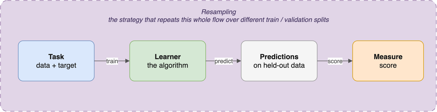
Each object owns one part of the workflow, and they snap together in a predictable way (Figure 26.1): a Learner trains on a Task to produce a fitted model, that model makes predictions, a Measure scores those predictions, and a Resampling strategy wraps the whole thing so the score reflects performance on data the model has never seen. Because all learners share the same interface, swapping classif.rpart for classif.ranger changes one string and nothing else.
ImportantWhy this design pays off
-
Consistency — every algorithm uses the same
train()/predict()interface, so there’s one set of habits to learn, not one per package. - Flexibility — mix and match tasks, learners, measures, and resamplings to run experiments by editing a single component.
- Reproducibility — randomness is controllable, so results are repeatable.
- Best practices baked in — the design nudges you toward train/test splitting and cross-validation rather than leaving them as an afterthought.
You’ve now met all four mlr3 building blocks on a problem you already understand. In the next chapter these pieces come together on real biological data — classifying cancer types from gene expression, predicting age from DNA methylation — where you’ll see a Learner actually train on a Task and have its predictions scored by a Measure under a Resampling. The concepts are the same; only the data gets bigger and more interesting.
26.9 Summary
You can now:
- Name the four core mlr3 objects and the single job each one does — Task (data + problem), Learner (algorithm), Measure (score), Resampling (validation strategy).
- Build a classification Task with
as_task_classif()and inspect it withtask$feature_namesandtask$target_names. - List available algorithms with
mlr_learners$keys(), create one withlrn(), and see its tunable dials withlearner$param_set$ids(). - Pick a Measure with
msr()and a Resampling strategy withrsmp(), and read what their printouts are telling you.
The payoff is the interchangeable-parts design: learn the four sockets once, and every algorithm in the mlr3 ecosystem plugs into them the same way.
26.10 Exercises
These exercises reuse the penguins. Recall that in the previous chapter we also framed a regression problem — predicting a penguin’s body_mass_g from its other measurements. Let’s set that up in mlr3.
-
Build a regression task. Create a regression task that predicts
body_mass_g, usingas_task_regr(). Confirm the target and list the features.NoteSolutiontask_mass <- as_task_regr(penguins, target = "body_mass_g") task_mass$target_names[1] "body_mass_g"task_mass$feature_names[1] "bill_depth_mm" "bill_length_mm" "flipper_length_mm" [4] "island" "sex" "species" [7] "year"as_task_regr()is the regression counterpart ofas_task_classif(). The target is now the continuousbody_mass_g, andspecieshas joined the feature list — any column that isn’t the target becomes a feature. -
Find regression learners. Query the registry for learners that work on a regression task, and show the first ten.
NoteSolutionregr_learners <- mlr_learners$keys("regr") head(regr_learners, 10)[1] "regr.cv_glmnet" "regr.debug" "regr.featureless" "regr.glmnet" [5] "regr.kknn" "regr.km" "regr.lm" "regr.nnet" [9] "regr.ranger" "regr.rpart"These are the
regr.*algorithms — for exampleregr.lm(linear regression) andregr.rpart(a regression tree). The naming convention tells you each one’s task type at a glance. -
Set up 10-fold cross-validation. Create a resampling object for 10-fold cross-validation and confirm the fold count from its parameter set.
NoteSolutioncv10 <- rsmp("cv", folds = 10) cv10$param_set$values$folds [1] 10rsmp("cv", folds = 10)builds the strategy;param_set$valuesreports the settings you actually chose, confirmingfoldsis 10. More folds give a more stable estimate of performance at the cost of more computation. -
Pick a regression measure. Create the root-mean-squared-error measure with
msr("regr.rmse")and print it. Does the framework want it minimized or maximized?NoteSolutionrmse_measure <- msr("regr.rmse") rmse_measure── <MeasureRegrSimple> (regr.rmse): Root Mean Squared Error ──────────────────── • Packages: mlr3 and mlr3measures • Range: [0, Inf] • Minimize: TRUE • Average: macro • Parameters: list() • Properties: weights and obs_loss • Predict type: response • Predict sets: test • Aggregator: mean()The printout shows
Minimize: TRUE— RMSE is an error, so smaller is better, and the framework will minimize it when comparing models. Contrast this with accuracy, which it maximizes.