24 Introduction to machine learning
Suppose you have gene-expression profiles from a hundred tumour biopsies and a hundred matched normal tissues, and a new, unlabelled sample arrives. Can you tell whether it is tumour or normal from its expression pattern alone? Or imagine you have DNA-methylation measurements from thousands of people of known age, and you want to estimate the biological age of someone new. These are not problems you can solve by sitting down and writing an explicit rule — there is no single gene, no simple if statement, that separates tumour from normal across every patient. The signal is spread across thousands of features in ways that are too subtle to codify by hand.
Machine learning is the set of tools for exactly this situation: instead of programming the rule yourself, you let an algorithm learn the rule from labelled examples, then apply it to new cases it has never seen. That last part — performing well on new data, not just the data you trained on — is the whole point. It is called generalization, and most of this chapter is really about how to get it and how to avoid fooling yourself into thinking you have it.
Machine learning in biology is a broad and fast-moving field. Greener et al. (2022) give an approachable overview of the methods used in biology, and Libbrecht and Noble (2015) review their early use in genetics and genomics. This chapter is the conceptual on-ramp: what machine learning is, the three families of problems it solves, the workflow you follow, and the single most important pitfall (overfitting) to watch for. The chapters that follow put these ideas to work — a tour of supervised algorithms on a shared dataset, the mlr3verse framework for running them cleanly, and worked biological examples — including the tumour-classification and age-from-methylation problems we just sketched.
24.1 What you’ll learn
- Recognize the three paradigms of machine learning — supervised, unsupervised, and reinforcement learning — and match a biological question to the right one.
- Distinguish classification (predicting a category) from regression (predicting a number) within supervised learning.
- Walk through the stages of a machine learning workflow, from problem definition to evaluation.
- Explain why you must split your data into training, validation, and test sets, and what each set is for.
- Recognize overfitting and underfitting, and describe how cross-validation and the bias–variance tradeoff help you steer between them.
24.2 The three kinds of machine learning
Machine learning problems come in a few distinct flavours, and the first skill to develop is recognizing which flavour you are facing. The flavour determines what data you need and what kind of answer you can expect.
Supervised learning is the most common in practice, and it covers most of the biological examples above. Here you have both the inputs (the features — gene expression values, methylation levels, clinical measurements) and the correct answers (the labels or targets — tumour vs normal, the patient’s age) for a set of training examples. The algorithm learns to map inputs to outputs by studying these example pairs. Supervised problems split further into two types:
- Classification predicts a category. Is this sample tumour or normal? Which of five cancer subtypes is this? The answer is one of a fixed set of labels.
- Regression predicts a number. What is this patient’s age? What is the expression level of this gene? The answer is a continuous value.
Unsupervised learning applies when you have the features but no labels — you do not have a known answer to predict. Instead, the algorithm looks for structure hidden in the data itself. Clustering groups similar samples together; you might cluster single cells by their expression profiles to discover cell types nobody labelled in advance. The k-means clustering chapter works through a complete clustering example on real yeast gene-expression data. Dimensionality reduction (like PCA) finds the few underlying factors that explain most of the variation across thousands of genes. These methods are often the first thing you reach for when you want to explore a new dataset before you commit to a specific prediction.
Reinforcement learning is a different shape of problem altogether. Rather than learning from a fixed pile of examples, an agent takes actions in an environment and receives rewards or penalties, improving its decisions through trial and error. It powers game-playing systems and robotics, and is appearing in areas like experimental design and molecule generation, but it needs specialized techniques and a lot of compute. We mention it for completeness; the rest of this part of the book focuses on supervised and unsupervised learning, which cover the great majority of everyday biological data analysis.
| Learning type | What you give it | What it gives back | Biological example |
|---|---|---|---|
| Supervised | Features and labels | Predicted labels/values | Tumour vs normal from expression; age from methylation |
| Unsupervised | Features only | Discovered structure | Clustering cells into types; PCA of samples |
| Reinforcement | An environment to act in | A decision policy | Sequential experiment design |
When thinking about machine learning, it can help to have a simple framework in mind. Figure 24.1 shows a tidy view of the field from the scikit-learn project, organized around the same questions: are you predicting a category, predicting a quantity, or looking for structure?
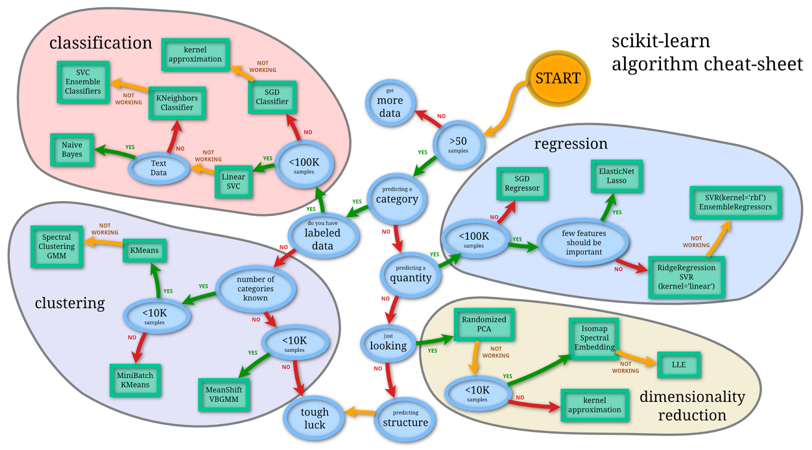
ml_map), © the scikit-learn developers, BSD 3-Clause.
- Data
- The foundation of machine learning. It can be structured (tabular) or unstructured (text, images, audio), and is usually divided into training, validation, and testing sets for model development and evaluation.
- Features
- The variables or attributes used to describe each data point (for example, the expression level of each gene). Feature engineering and selection are crucial steps for improving model performance and interpretability.
- Models and algorithms
- A model is a mathematical representation of the relationship between features and the target. An algorithm is the method used to fit a model to data, such as linear regression, decision trees, and neural networks.
- Hyperparameters and tuning
- Hyperparameters are adjustable settings that control the learning process (for example, how deep a decision tree may grow). Tuning is the search for the values that give the best performance.
- Evaluation metrics
- Numbers that quantify how well a model does — accuracy, precision, recall, and F1-score for classification; mean squared error and R-squared for regression.
24.3 The machine learning workflow
Successful machine learning projects follow a structured workflow. The process begins long before any algorithm is trained and extends well beyond the first model you fit.
- Problem definition — state clearly what you want to predict and decide whether machine learning is even the right tool.
- Data collection and preparation — gather relevant data and clean it into a form a model can use.
- Data splitting — divide the data into training, validation, and test sets so you can evaluate honestly.
- Model selection — choose an algorithm and configure its hyperparameters.
- Training — fit the model to the training data so it can learn the patterns.
- Evaluation — measure performance on held-out data using appropriate metrics.
- Deployment — put the model to work on new, real data.
The journey starts with problem definition. You need to articulate what you are trying to achieve and whether machine learning is the appropriate solution. Not every problem needs it; sometimes a simple statistical test or a known biological rule gives a better answer with far less complexity.
Data collection and preparation usually consume most of the time in a real project. Raw data rarely arrives ready to model. You will spend effort handling missing values, encoding categorical variables, scaling numerical features, and dealing with outliers and batch effects. The quality of this preparation often decides whether the whole project succeeds.
Data splitting deserves special attention because it directly controls how trustworthy your results are. The training set teaches the algorithm, but if you then judge performance on that same data, you get a flattering picture that will not hold up on new samples. It is like letting students see the exam questions while they study, then grading them on those exact questions.
Splitting your data into separate sets is the foundation of honest evaluation, and it is the single best defence against fooling yourself.
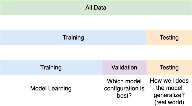
- Training data is used to fit the model’s parameters.
- Validation data helps you choose between models and tune hyperparameters.
- Test data gives a final, unbiased estimate of performance on new data.
The golden rule: never use the test data for any decision during model development. Reserve it for the final evaluation only.
A common starting point is an 80% training / 20% testing split. For more involved projects, a three-way split might use 60% for training, 20% for validation (model selection), and 20% for final testing. Cross-validation, which we return to below, offers a more data-efficient alternative while still keeping a test set untouched.
k in k-nearest neighbours) as well as their parameters (like the slopes in linear regression), a separate validation set is essential.
Model selection means choosing both the type of algorithm and its specific settings. Different algorithms make different assumptions and shine in different situations. Linear models work well when relationships are roughly linear and you value interpretability. Tree-based methods handle nonlinear relationships and interactions naturally but can overfit with limited data. Neural networks can capture very complex patterns but need large datasets and careful tuning. Hyperparameters describe the shape of the model — the depth of a decision tree, the k in k-nearest neighbours, the learning rate in gradient descent — and hyperparameter tuning is the search for good values, often using grid or random search together with cross-validation.
Training is where the algorithm actually learns. The model adjusts its internal parameters to reduce its errors on the training set. But the goal is not a perfect score on the training data; a model that fits the training data too closely often fails on new examples, a problem called overfitting.
Evaluation tells you whether the model is ready. This means looking past a single accuracy number — precision, recall, and F1-score for classification, or mean squared error and R-squared for regression — and checking that performance holds up across the different subgroups in your data.
24.4 Overfitting and underfitting
Recall that the goal is a model that generalizes well to new, unseen data. Given enough flexibility, almost any model can fit the data it was trained on perfectly. The real challenge is balancing a good fit on the training data against good performance on new examples — and it is that second part, generalization, that we actually care about.
When a model overfits, it learns the training data too well, memorizing the specific examples instead of the general pattern. The result is excellent performance on training data and poor performance on anything new.
A familiar analogy: imagine teaching someone to recognize cats by showing them 100 photos. An overfitted learner memorizes every pixel of those particular photos rather than learning the general features — whiskers, pointed ears, fur. Shown a new cat, they are lost, because they fixated on details unique to the training images. The genomics version is the same story: a model that learns to separate your 200 tumour and normal samples by latching onto a few quirks of those 200 patients (or a batch effect in that sequencing run) will collapse the moment you hand it samples from a new hospital.
Underfitting is the opposite failure. An underfitted model is too simple to capture the real pattern, so it does poorly on both training and new data. In the cat analogy, an underfitted model might only look at overall image brightness and miss every feature that actually distinguishes a cat.
Code
set.seed(123)
sinsim <- function(n, sd = 0.1) {
  x <- seq(0, 1, length.out = n)
  y <- sin(2 * pi * x) + rnorm(n, 0, sd)
  return(data.frame(x = x, y = y))
}
dat <- sinsim(100, 0.25)
library(ggplot2)
library(patchwork)
p_base <- ggplot(dat, aes(x = x, y = y)) +
  geom_point(alpha = 0.7) +
  theme_bw()
p_lm <- p_base +
  geom_smooth(method = "lm", se = FALSE, alpha = 0.6, formula = y ~ x)
p_lmsin <- p_base +
  geom_smooth(method = "lm", formula = y ~ sin(2 * pi * x), se = FALSE, alpha = 0.6)
p_loess_wide <- p_base +
  geom_smooth(method = "loess", span = 0.5, se = FALSE, alpha = 0.6, formula = y ~ x)
p_loess_narrow <- p_base +
  geom_smooth(method = "loess", span = 0.05, se = FALSE, alpha = 0.6, formula = y ~ x)
p_lm + p_lmsin + p_loess_wide + p_loess_narrow + plot_layout(ncol = 2) +
  plot_annotation(tag_levels = "A") &
  theme(plot.tag = element_text(size = 8))
Warning in simpleLoess(y, x, w, span, degree = degree, parametric = parametric,
: k-d tree limited by memory. ncmax= 200Warning in sqrt(sum.squares/one.delta): NaNs produced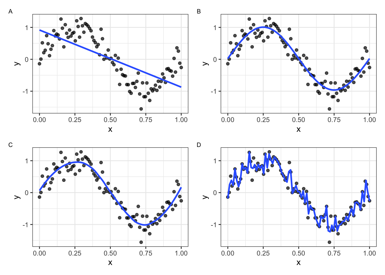
In Figure 24.3 we simulate data from the function \(f(x) = sin(2 \pi x) + N(0,0.25)\) and fit four models of increasing flexibility. A model that is too simple (A) underfits: the straight line cannot follow the wave at all. A model that is too flexible (D) overfits: the narrow-span loess curve chases every wiggle of the random noise instead of the smooth trend beneath it. Models (B) and (C) sit in the sweet spot — flexible enough to capture the real pattern, restrained enough to ignore the noise.
The relationship between model complexity and performance tends to follow a U shape. Very simple models do badly because they underfit. As you add complexity, performance improves as the model captures more of the real signal. But past an optimal point, extra complexity starts fitting noise, and performance on new data gets worse again. Figure 24.4 draws this out — the two curves are the heart of the whole chapter.
Code
library(ggplot2)
complexity <- seq(0.5, 10, length.out = 300)
train_err  <- 0.85 / (complexity^0.75) + 0.04         # falls monotonically
test_err   <- 0.85 / complexity + 0.018 * complexity  # U-shaped
df <- data.frame(
  complexity = rep(complexity, 2),
  error      = c(train_err, test_err),
  set        = rep(c("Training error", "Error on new data"), each = length(complexity))
)
best <- complexity[which.min(test_err)]
ggplot(df, aes(complexity, error, colour = set)) +
  geom_vline(xintercept = best, linetype = "dashed", colour = "grey55") +
  geom_line(linewidth = 1.2) +
  annotate("text", x = best, y = 0.60, label = "sweet spot", colour = "grey30",
           fontface = "italic", size = 3.4) +
  annotate("text", x = 1.0, y = 0.70, label = "underfitting", colour = "grey30",
           hjust = 0, size = 3.4) +
  annotate("text", x = 9.6, y = 0.40, label = "overfitting", colour = "grey30",
           hjust = 1, size = 3.4) +
  scale_colour_manual(values = c("Training error"   = "#6c8ebf",
                                 "Error on new data" = "#b85450")) +
  labs(x = "Model complexity →", y = "Prediction error →", colour = NULL) +
  theme_bw() +
  theme(axis.text = element_blank(), axis.ticks = element_blank(),
        legend.position = "top", panel.grid.minor = element_blank())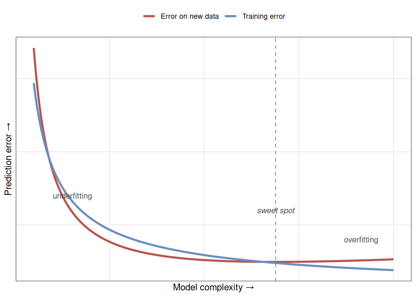
Overfitting shows up as a widening gap between training and validation performance. If your model scores 95% accuracy on training data but only 70% on validation data, it is almost certainly overfitting.
Watch both numbers throughout development. The best models perform similarly on training and validation data — a sign they have learned the pattern, not the particular examples.
Several strategies push back against overfitting. Regularization adds a penalty for complexity, nudging the model toward simpler solutions. Cross-validation (next section) gives more reliable performance estimates by validating on several data splits. Early stopping halts training once validation performance starts to slip. Feature selection trims the input down to the variables that actually matter — often crucial in genomics, where you may start with tens of thousands of genes.
The bias–variance tradeoff is the theory behind all of this, and the cleanest way to feel it is a thought experiment. Imagine you could repeat your whole study many times over — each time recruiting a fresh sample of patients from the same population and refitting your model from scratch. Two very different kinds of error can show up across those repeats.
Bias is the error that survives the repetition: the part the model gets wrong systematically, the same way every time, no matter which sample it drew. It is the signature of a model too simple to capture the real relationship. Picture trying to fit a straight line to an epigenetic clock whose methylation-versus-age relationship genuinely curves — every sample produces a line that misses the bend in the same direction. The model is the wrong shape, so more data cannot rescue it. High bias is underfitting.
Variance is the opposite failure: how much the fitted model jumps around from one sample to the next. A very flexible model — a deep decision tree, say — will contort itself to the particular handful of patients it trained on, fitting their noise as if it were signal. Give it a different sample of the same size and you get a noticeably different model that makes different predictions for the very same new patient. The model is too sensitive to the luck of the draw. High variance is overfitting.
A dartboard makes the contrast concrete. A high-bias thrower lands every dart in a tight cluster, but off to one side of the bullseye — consistent, and consistently wrong. A high-variance thrower sprays darts all around the board — occasionally dead-on, but unreliable. You want neither: you want a tight cluster at the centre.
Here is the catch that makes it a tradeoff: pushing one error down tends to push the other up. A simpler model has low variance but high bias; a more complex one trades the reverse. The model that generalizes best is the one that balances these two competing sources of error. Figure 24.5 shows why: the error on new data is essentially bias plus variance, and because one falls as the other rises, their sum traces the very U we saw above.
Code
library(ggplot2)
x        <- seq(0, 10, length.out = 400)
bias2    <- exp(-0.5 * x)              # high for simple models, falls with complexity
variance <- 0.01 * exp(0.5 * x)        # low for simple models, rises with complexity
floor    <- 0.12                       # irreducible error (noise we can never remove)
total    <- bias2 + variance + floor   # expected error on new data
opt      <- x[which.min(total)]        # complexity that minimises total error

df <- data.frame(
  x     = rep(x, 3),
  error = c(total, variance, bias2),
  curve = factor(rep(c("Total error", "Variance", "Bias²"), each = length(x)),
                 levels = c("Total error", "Variance", "Bias²"))
)
cols <- c("Total error" = "#1a1a1a", "Variance" = "#3a9aa5", "Bias²" = "#a8322a")

ggplot(df, aes(x, error, colour = curve)) +
  # axes drawn as arrows, like a hand-sketched schematic
  annotate("segment", x = 0, xend = 0, y = 0, yend = 1.72,
           arrow = arrow(length = unit(0.22, "cm"), type = "closed"), linewidth = 0.5) +
  annotate("segment", x = 0, xend = 10.7, y = 0, yend = 0,
           arrow = arrow(length = unit(0.22, "cm"), type = "closed"), linewidth = 0.5) +
  # optimum complexity marker
  annotate("segment", x = opt, xend = opt, y = 0, yend = 1.5,
           linetype = "dotted", colour = "grey25", linewidth = 0.5) +
  annotate("point", x = opt, y = 0, shape = 21, fill = "white",
           colour = "black", size = 2.6, stroke = 0.7) +
  annotate("text", x = opt - 0.18, y = 1.02, label = "Optimum Model Complexity",
           angle = 90, fontface = "italic", size = 3.2, colour = "grey20") +
  geom_line(linewidth = 1.1) +
  # curve labels
  annotate("text", x = 6.1,  y = 1.34, label = "Total Error", colour = cols[["Total error"]], size = 3.8) +
  annotate("text", x = 8.9,  y = 0.78, label = "Variance",    colour = cols[["Variance"]],    size = 3.8) +
  annotate("text", x = 8.9,  y = 0.14, label = "Bias²",  colour = cols[["Bias²"]],  size = 3.8) +
  scale_colour_manual(values = cols) +
  scale_x_continuous(expand = c(0, 0)) +
  scale_y_continuous(expand = c(0, 0)) +
  coord_cartesian(xlim = c(-0.8, 10.9), ylim = c(-0.2, 1.8), clip = "off") +
  annotate("text", x = 5.3, y = -0.16, label = "Model Complexity", size = 4) +
  annotate("text", x = -0.62, y = 0.85, label = "Error", angle = 90, size = 4) +
  theme_void() +
  theme(legend.position = "none", plot.margin = margin(6, 12, 8, 18))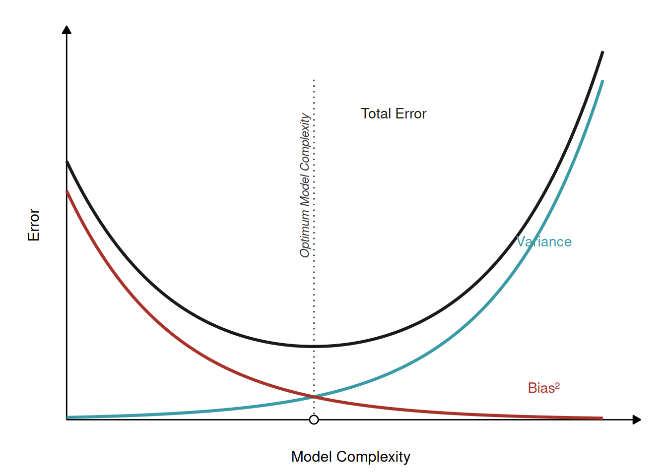
24.5 Cross-validation and model selection
Cross-validation answers a practical question: how do you reliably estimate a model’s performance when you only have so much data? A single train–test split can mislead you, especially with small datasets, because the estimate depends heavily on which samples happen to land in which set.
K-fold cross-validation is the standard fix. You split the training data into k equal parts (folds). You then train the model k times; each time, one fold is held out for validation and the other k − 1 are used for training. Averaging the k resulting scores gives a much steadier estimate of model quality than any single split. Figure 24.6 shows the rotation for k = 5.
Code
library(ggplot2)
k <- 5
grid <- expand.grid(fold = 1:k, round = 1:k)
grid$role <- ifelse(grid$fold == grid$round, "Validation", "Train")
ggplot(grid, aes(x = fold, y = round, fill = role)) +
  geom_tile(colour = "white", linewidth = 3) +
  geom_text(aes(label = role), size = 2.9, colour = "grey25") +
  scale_fill_manual(values = c("Train" = "#dae8fc", "Validation" = "#ffe6cc")) +
  scale_x_continuous(breaks = 1:k, labels = paste("Fold", 1:k), position = "top",
                     expand = c(0, 0)) +
  scale_y_reverse(breaks = 1:k, labels = paste("Round", 1:k), expand = c(0, 0)) +
  coord_equal() +
  labs(x = NULL, y = NULL, fill = NULL) +
  theme_minimal() +
  theme(legend.position = "none", panel.grid = element_blank(),
        axis.text = element_text(colour = "grey25"))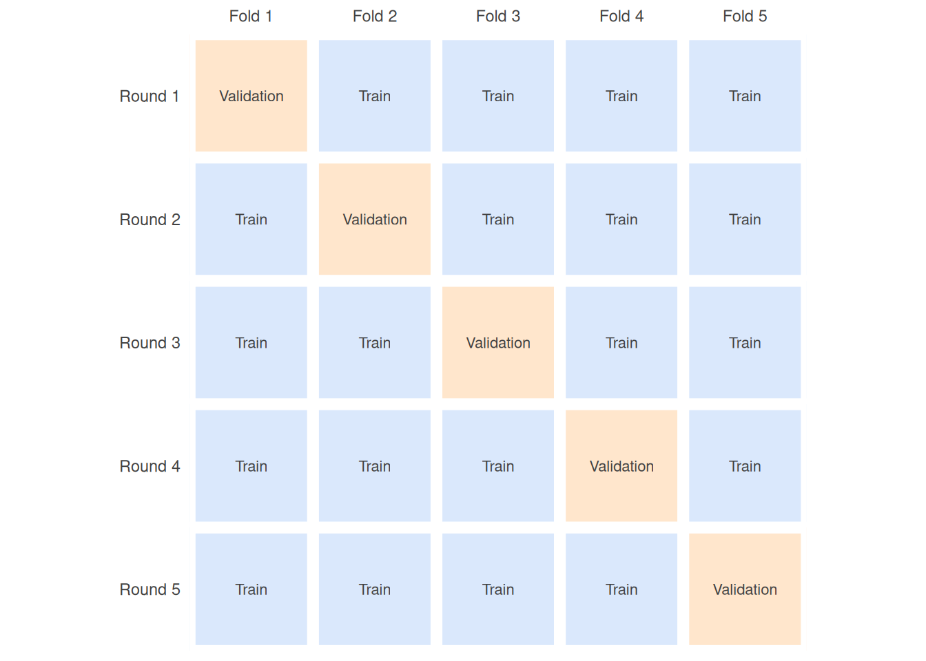
Five-fold and ten-fold cross-validation are the usual choices, trading off computation against reliability. Leave-one-out cross-validation is the extreme case where k equals the number of training examples — it uses the data maximally but can be slow and, for some models, overly optimistic.
A couple of biological wrinkles are worth flagging. Stratified cross-validation keeps the same proportion of each class in every fold, which matters whenever your classes are imbalanced — say, many more normal samples than tumours. And when samples are not independent — repeated measures from the same patient, or cells from the same donor — you must keep related samples together in the same fold, or the model can “peek” and your estimate becomes too rosy.
Cross-validation does triple duty: it helps you pick the best algorithm from a set of candidates, tune hyperparameters within an algorithm, and estimate realistic performance on new data. But remember the golden rule from earlier — every one of those cross-validation results still comes from the training data. The final verdict always comes from a completely separate test set.
24.6 Exercises
These are concept-checking exercises; no coding required. Try each one before opening the solution.
-
Name the paradigm and the task. For each scenario, say whether it is supervised, unsupervised, or reinforcement learning. If it is supervised, say whether it is classification or regression.
- You have RNA-seq profiles from 300 breast-tumour samples, each labelled with one of four molecular subtypes, and you want to assign subtypes to new tumours.
- You have DNA-methylation profiles from 1,000 people of known chronological age, and you want to predict the age of a new person.
- You have single-cell expression profiles from a tissue with no prior labels, and you want to discover how many distinct cell populations are present.
NoteSolution- Supervised, classification — the answer is one of a fixed set of categories (the four subtypes).
- Supervised, regression — age is a continuous number.
- Unsupervised (clustering) — there are no labels to predict; you are discovering structure in the data.
-
Spot the leakage. A colleague reports 99% accuracy classifying tumour vs normal. You discover they tuned the model and reported accuracy on the same set of samples. What is wrong, and what should they have done instead?
NoteSolutionThey evaluated on data the model had already seen during development, so the 99% is optimistic and will not hold on new samples — exactly the “exam questions seen while studying” trap. They should have held out a test set that played no role in training or tuning, and reported accuracy on that. Cross-validation on the training portion could guide the tuning, but the final number must come from the untouched test set.
-
Underfit or overfit? During development you see 98% accuracy on the training data but only 62% on the validation data. Is this underfitting or overfitting? Name one thing you could try.
NoteSolutionThis large train-versus-validation gap is the signature of overfitting: the model has learned the training examples rather than the general pattern. You could add regularization, select fewer features, choose a simpler model, or gather more training data. (Underfitting would instead show poor scores on both sets.)
-
Why fold at all? You have only 80 labelled samples. Why might five-fold cross-validation give you a more trustworthy performance estimate than a single 80/20 train–test split?
NoteSolutionWith only 80 samples, a single test set of 16 is small, and its score depends heavily on which samples happen to land in it. Five-fold cross-validation lets every sample serve as validation data exactly once and averages five estimates, giving a steadier, less luck-dependent picture of how the model performs.
24.7 Summary
You can now place a biological question into the right machine-learning family — supervised when you have labelled examples to predict from (and within that, classification for categories, regression for numbers), unsupervised when you are exploring unlabelled data for structure, and reinforcement for learning by interaction. You have walked the workflow from problem definition through data preparation, splitting, model selection, training, and evaluation, and you understand why the test set must stay untouched until the very end. You can recognize overfitting and underfitting, read them off the gap between training and validation scores, and explain how cross-validation and the bias–variance tradeoff help you find the model that generalizes.
With these concepts in hand, you are ready for the tour of supervised algorithms, where each of these ideas becomes runnable R code on real biological data.