21 Working with distribution functions

Author

Affiliation

University of Colorado
Anschutz School of Medicine

Published

June 1, 2024

Modified

June 11, 2026

Heights, blood pressures, measurement errors, log-transformed gene-expression values — measure enough of almost anything in biology and the values tend to pile up into the same bell-shaped curve: the normal distribution. Once your data follow that curve, you’ll want to ask questions of it. What fraction of samples fall below some cutoff? Which value marks the top 5%? Give me twenty random draws to simulate an experiment. R answers each of those with a different function.

The catch is remembering which function does which job. This chapter is a visual guide: for every function we pair the R call with a picture of exactly what it measures on the bell curve, because the difference between a probability, a density, and a quantile is far easier to see than to memorize. It’s genuinely hard to reason about these functions without a shape to point at — so a shape is what we’ll build for each one.

21.1 What you’ll learn

Use pnorm() to turn a value into a probability (the area under the curve to its left).
Use dnorm() to get the height (density) of the curve at a value.
Use qnorm() to go the other direction — from a probability back to a value.
Use rnorm() to draw random samples from a normal distribution.
Combine these functions to answer real questions about normally distributed data, such as IQ scores.

One naming rule for every distribution

R builds these names from a one-letter prefix plus the distribution: d for density, p for probability, q for quantile, r for random. Learn it once and it transfers everywhere — dbinom/pbinom/qbinom/rbinom for the binomial, dt/pt/qt/rt for the t-distribution we meet in the next chapter, dpois/ppois/… for the Poisson. Here we use the …norm family for the normal.

The four functions, at a glance:

Function	Input	Output
`pnorm`	a value `q`	P(X < q): area under the curve to the left of `q`
`dnorm`	a value `x`	the height of the density curve at `x`
`qnorm`	a probability from 0 to 1	the value `x` where P(X < x) equals that probability
`rnorm`	a count `n`	`n` random samples from the distribution

Table 21.1: Functions for the normal distribution

In one sentence each: pnorm gives the area to the left of a point, dnorm gives the height of the curve at a point, qnorm is the inverse of pnorm (probability back to value), and rnorm generates random samples. The rest of the chapter unpacks them one at a time.

21.2 pnorm

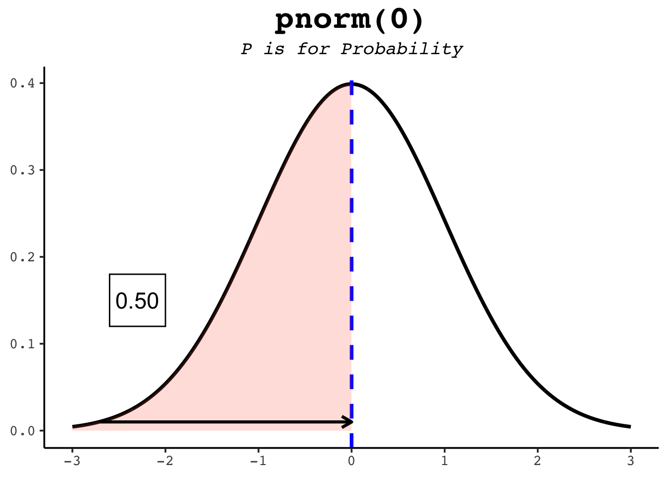
pnorm answers the question “what fraction of the distribution lies to the left of this value?” If you don’t supply a mean and standard deviation, R assumes the standard normal (mean 0, standard deviation 1). The help page gives this template:

pnorm(q, mean = 0, sd = 1, lower.tail = TRUE, log.p = FALSE)

You hand it q, a value on the x-axis, and it returns the area under the curve to the left of that point. The mean sits dead centre and splits the curve in half, so:

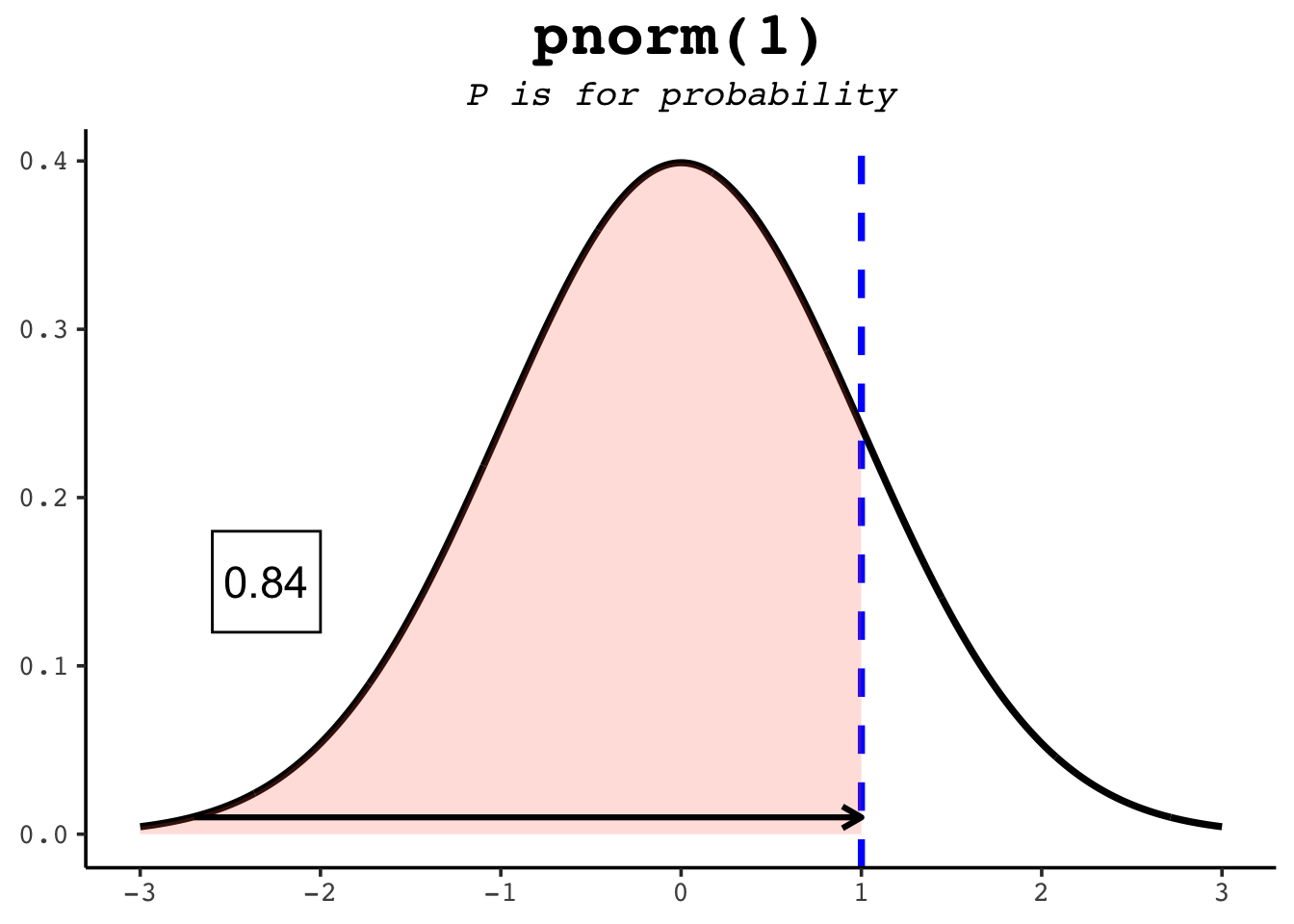
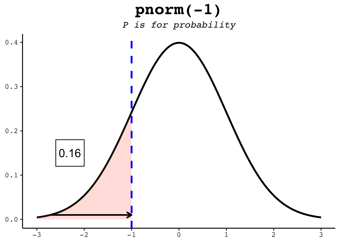
pnorm(0)    # half the distribution is below the mean

[1] 0.5

pnorm(1)    # ~84% is below one standard deviation above the mean

[1] 0.8413447

pnorm(-1)   # ~16% is below one standard deviation below it

[1] 0.1586553

The figures below show each of those as a shaded area.

Figure 21.1: The pnorm function takes a quantile (value on the x-axis) and returns the area under the curve to the left of that value.

Figure 21.2: The pnorm function takes a quantile (value on the x-axis) and returns the area under the curve to the left of that value.

Figure 21.3: The pnorm function takes a quantile (value on the x-axis) and returns the area under the curve to the left of that value.

Figure 21.4: The pnorm function takes a quantile (value on the x-axis) and returns the area under the curve to the left of that value.

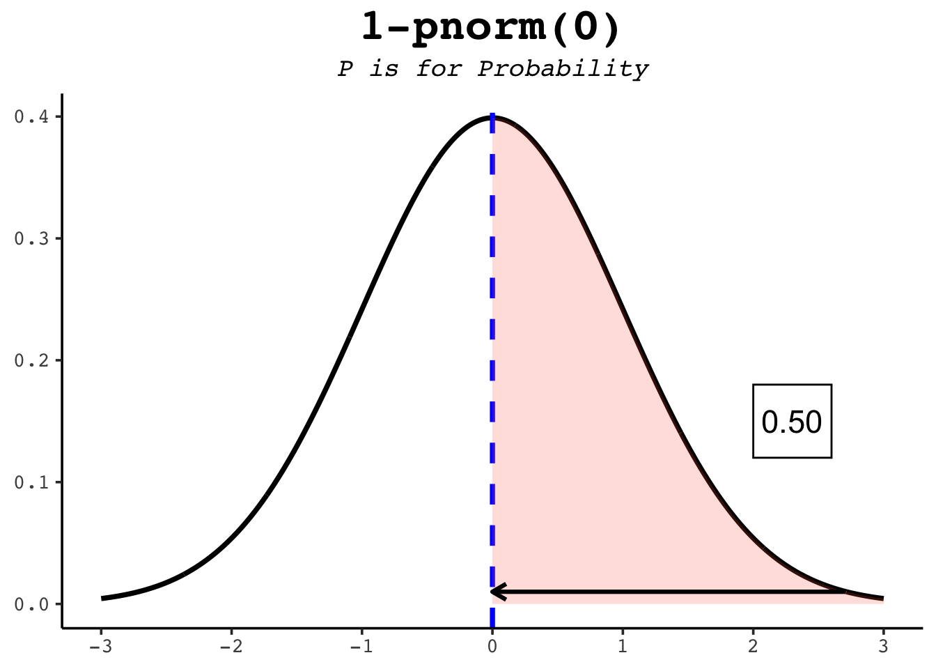
The option lower.tail = TRUE tells R to use the area to the left of the given point — the default. To get the area to the right instead, either switch to lower.tail = FALSE or subtract from 1:

pnorm(1, lower.tail = FALSE)   # area to the RIGHT of 1

[1] 0.1586553

1 - pnorm(1)                   # exactly the same thing

[1] 0.1586553

21.3 The cumulative distribution function

Step back and look at what pnorm really is. Each call answers one question — “how much probability lies to the left of this value?” If you ask that question at every point along the x-axis and plot the answers, you trace out a single curve: the cumulative distribution function, or CDF. Where the density (dnorm) tells you how concentrated probability is at each point, the CDF tells you how much has accumulated by that point. They are two views of the same distribution, and learning to move between them is most of what “distribution intuition” really means.

Here is the CDF of the standard normal — pnorm(x) evaluated at every x:

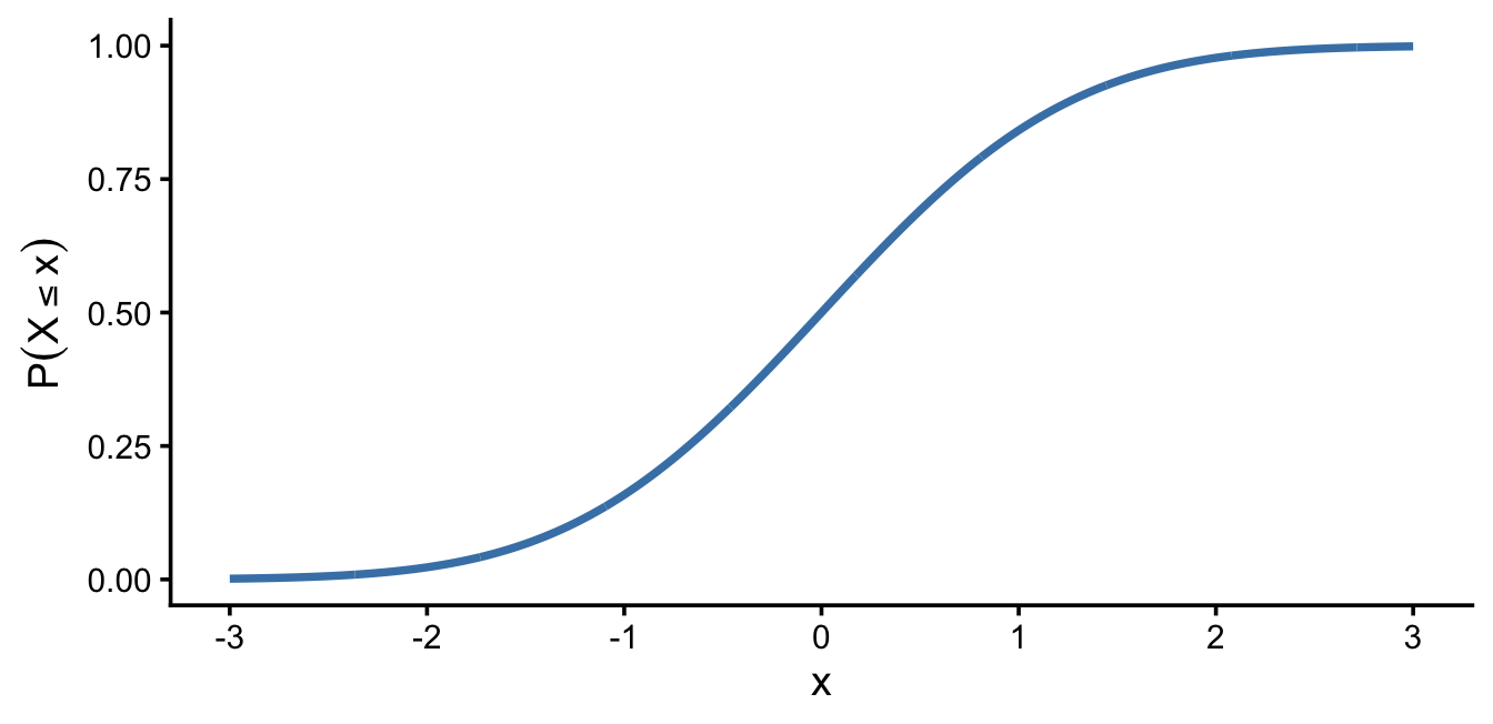
Figure 21.5: The cumulative distribution function of the standard normal: pnorm(x) plotted at every x. It is the running total of the area under the density curve, climbing from 0 (no probability accumulated yet) to 1 (all of it).

A few features are worth naming, because they hold for every CDF, not just the normal:

It starts near 0 and ends near 1. A CDF is accumulated probability, and all the probability sums to 1, so the curve can only climb from 0 up to 1.
It never goes down. Moving to the right can only add area, never remove it, so a CDF is always non-decreasing.
It is S-shaped (for the normal) because of where the density lives. Out in the left tail almost no probability is accumulating, so the curve is nearly flat; through the middle — where the bell is tallest — probability piles up quickly and the curve climbs steeply; in the right tail there is little left to add, so it levels off toward 1.

That last point is the key link between the two views: the density is the slope of the CDF. The curve rises fastest exactly where the density is tallest (the mean), and flattens wherever the density is near zero (the tails). Read the other direction, the CDF is the running total — the accumulated area — of the density.

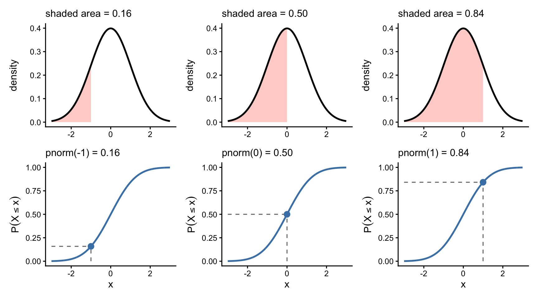
21.3.1 The area is the height

The cleanest way to feel the connection is to put the two pictures side by side. In Figure 21.6 the same value q appears in both rows: the shaded area under the density (top) is exactly the height of the CDF (bottom). As q slides to the right, the shading fills in and the point climbs the S-curve. That shaded area-equals-curve-height is precisely the number pnorm(q) returns.

Figure 21.6: Two views of the same probability at q = -1, 0, and 1. Top row: the density with the area to the left of q shaded. Bottom row: the CDF, with a point at (q, pnorm(q)) and dashed guides. In every column the shaded area above equals the height below.

21.3.2 Everything you already know, on one curve

Once you can see the CDF as a curve, the whole d/p/q/r family lines up on it:

pnorm reads the curve upward: hand it a value q on the x-axis and it returns the height of the curve there — the probability to the left.
qnorm reads the same curve across: hand it a probability on the y-axis and it returns the x where the curve reaches that height. That is why qnorm is the exact inverse of pnorm — it’s the same S-curve, read sideways.
dnorm is the curve’s steepness — how fast probability is piling up at that point.

So pnorm and qnorm are not two separate things to memorize; they are the same curve approached from two directions, and dnorm is its slope.

This isn’t special to the normal

Everything in this section is general. Every distribution — binomial, Poisson, t, exponential, and the rest — has a density (or, for counts, a probability mass) and a matching CDF, related in exactly the same way: the CDF is the accumulated area under the density, and the density is the slope of the CDF. That shared structure is why R gives every distribution the same d/p/q/r quartet. Swap norm for pois or binom and the picture you just built still holds.

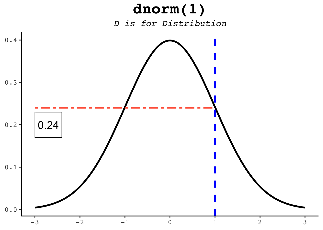
21.4 dnorm

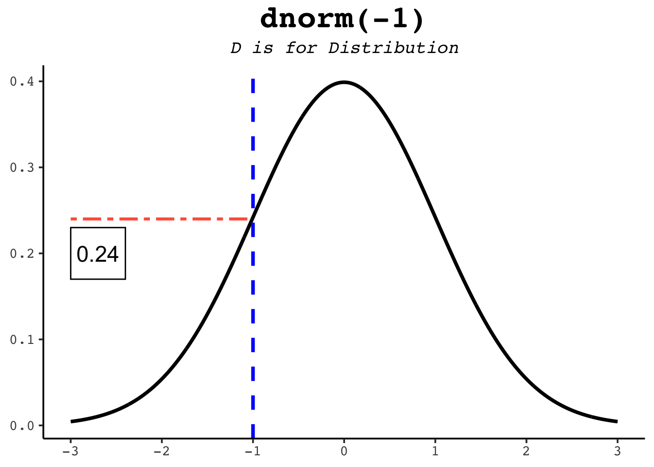
dnorm gives the height of the bell curve at a value — the probability density. The curve is tallest at the mean and falls off symmetrically on either side. Unlike pnorm, the result is not a probability you can read as a percentage; it’s the height of the curve, used mainly for drawing the distribution or in likelihood calculations.

dnorm(0)    # the peak of the standard normal

[1] 0.3989423

dnorm(1)    # lower, one SD out...

[1] 0.2419707

dnorm(-1)   # ...and the same height on the other side, by symmetry

[1] 0.2419707

The figures below mark each of these heights on the curve.

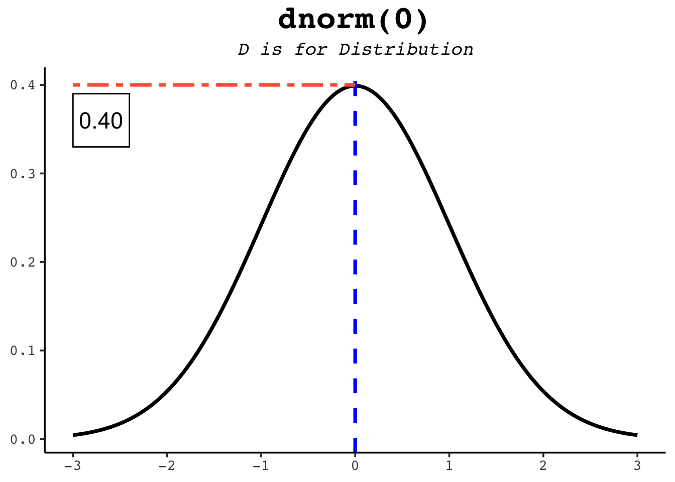
Figure 21.7: The `dnorm` function returns the height of the normal distribution at a given point.

Figure 21.8: The `dnorm` function returns the height of the normal distribution at a given point.

Figure 21.9: The `dnorm` function returns the height of the normal distribution at a given point.

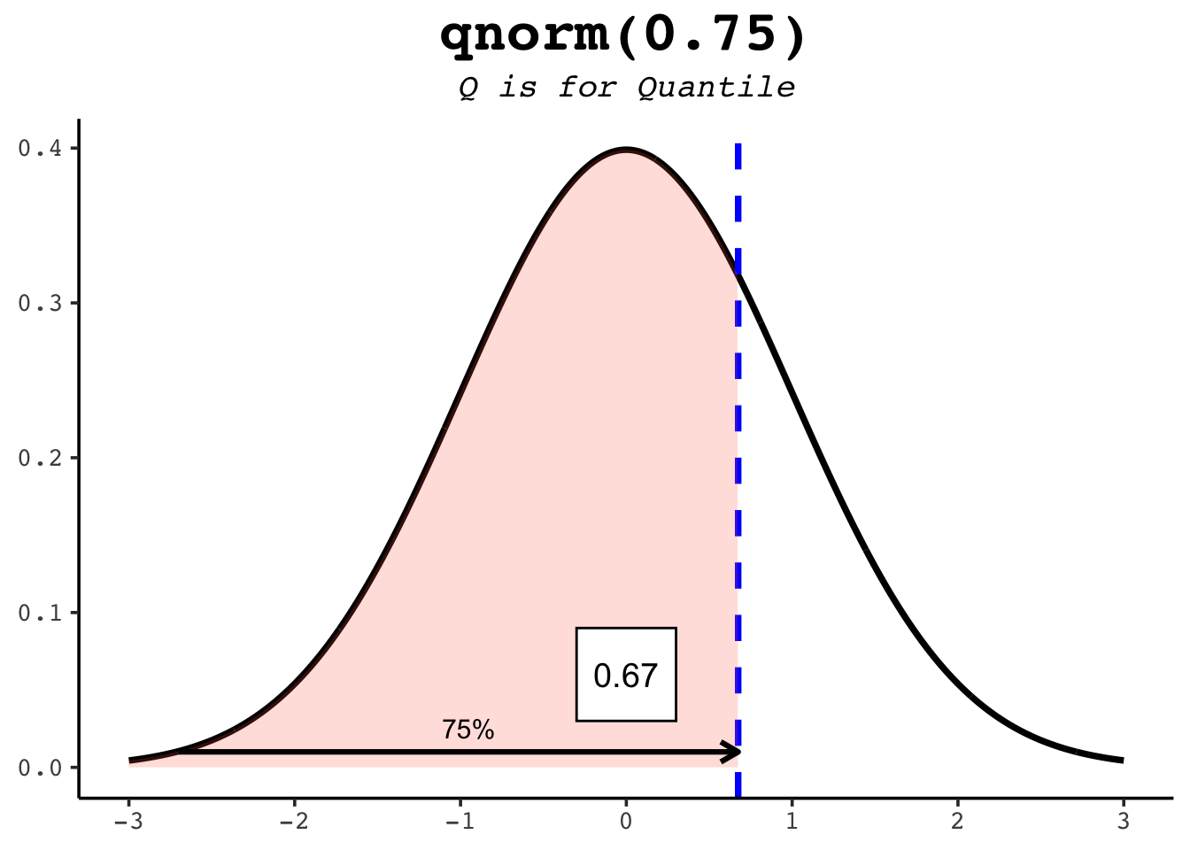
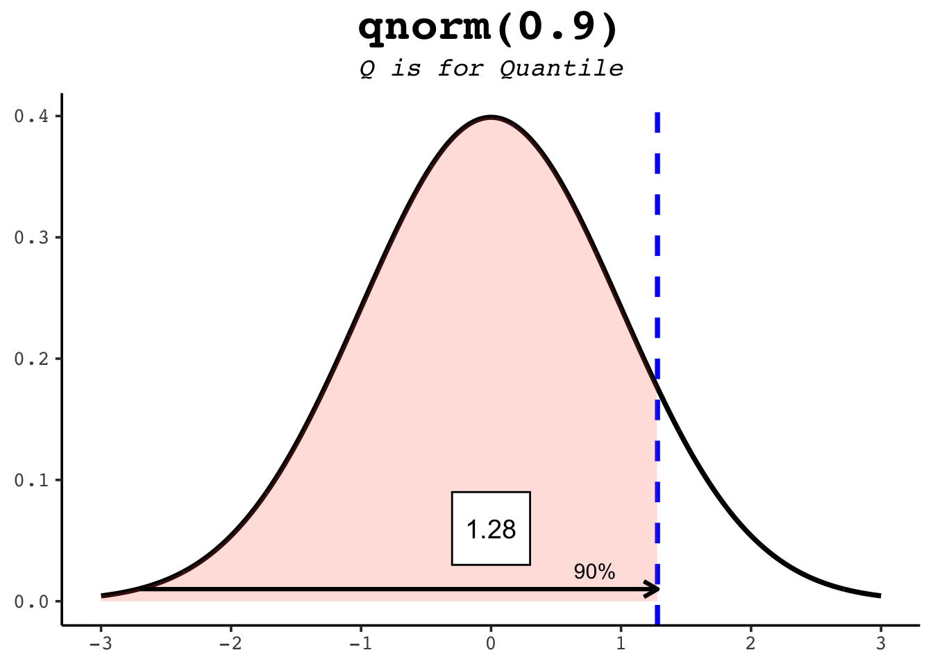
21.5 qnorm

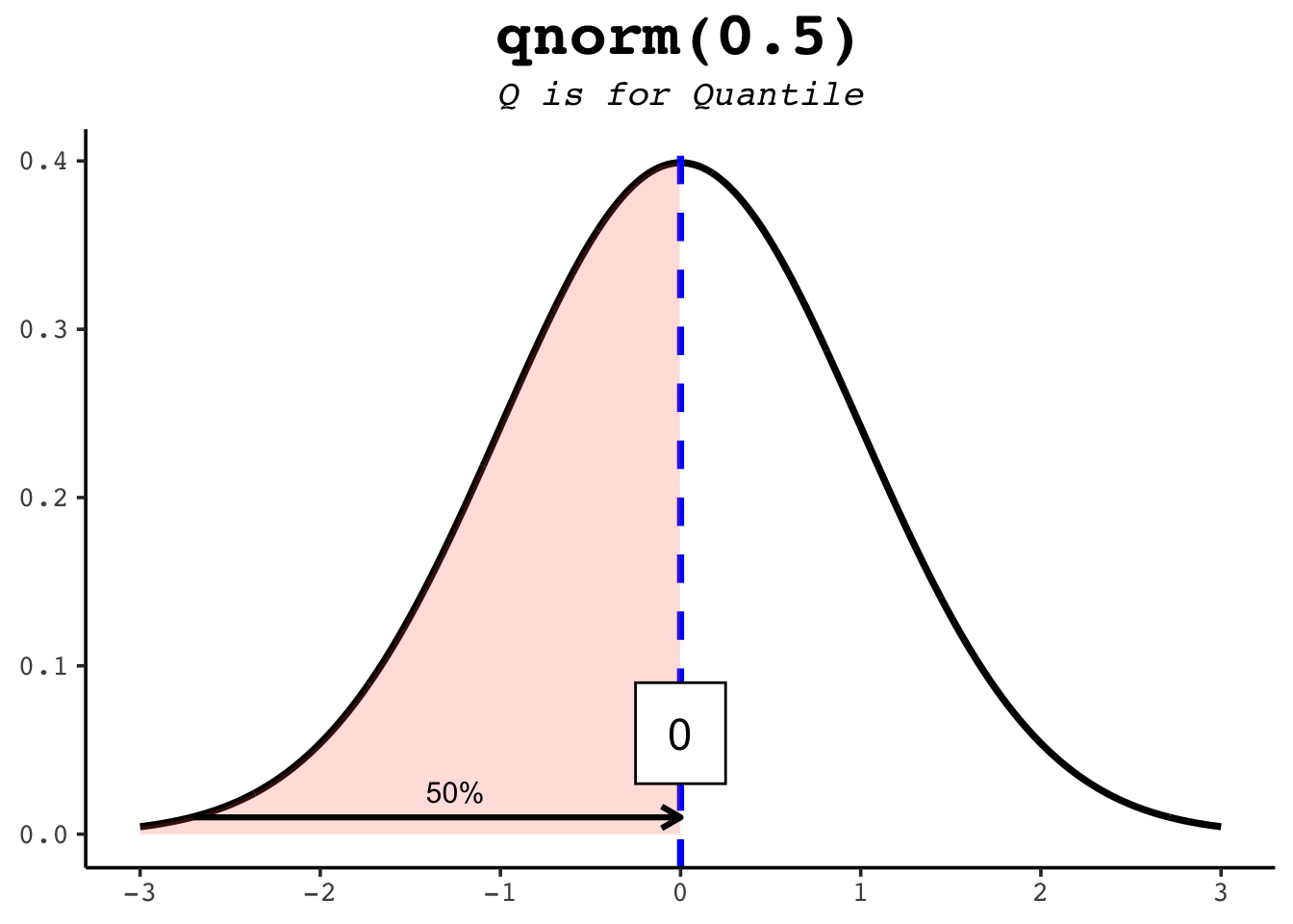
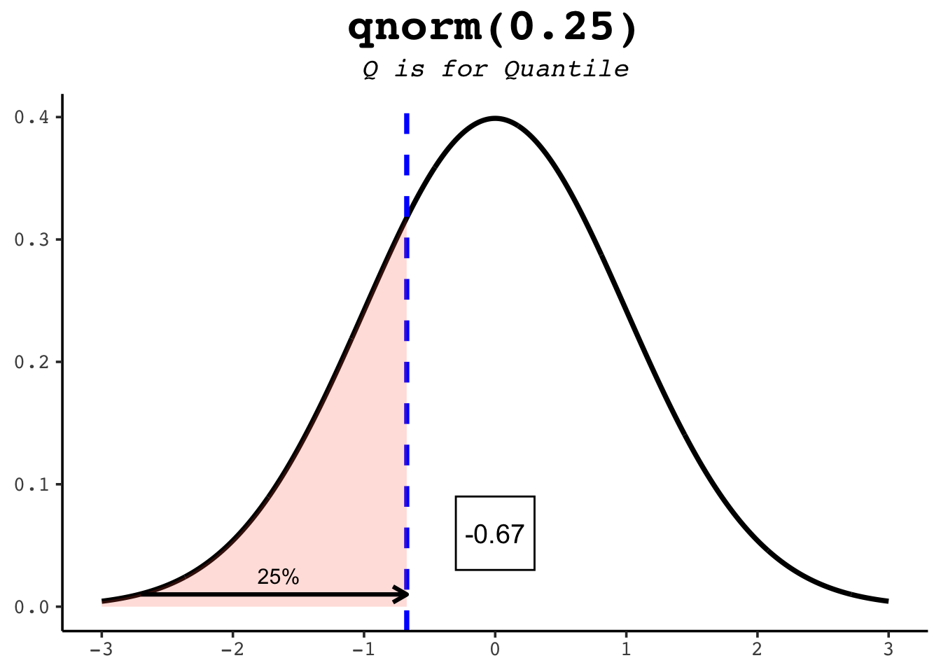
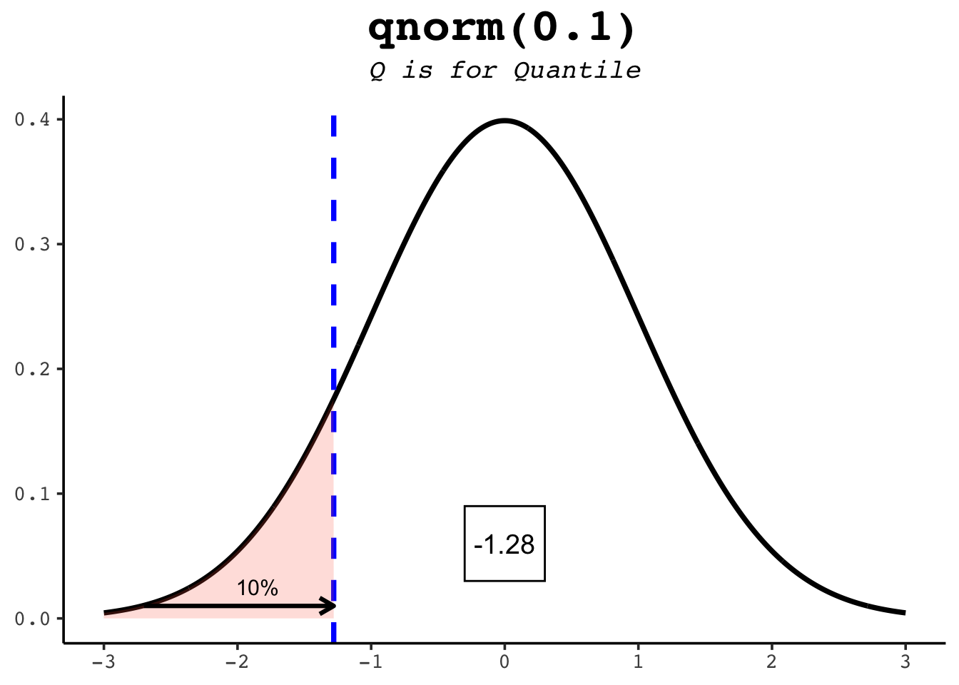
qnorm runs pnorm in reverse: hand it a probability and it returns the value with that much area to its left. Since pnorm(1) is about 0.84, qnorm(0.84) is about 1 — the two functions undo each other. This is how you find percentiles.

qnorm(0.5)     # the median: half the area lies to its left

[1] 0

qnorm(0.25)    # the first quartile

[1] -0.6744898

qnorm(0.975)   # the value cutting off the top 2.5% — the famous 1.96

[1] 1.959964

The figures below show several quantiles as shaded areas.

Figure 21.10: The qnorm function is the inverse of the pnorm function in that it takes a probability and gives the quantile.

Figure 21.11: The qnorm function is the inverse of the pnorm function in that it takes a probability and gives the quantile.

Figure 21.12: The qnorm function is the inverse of the pnorm function in that it takes a probability and gives the quantile.

Figure 21.13: The qnorm function is the inverse of the pnorm function in that it takes a probability and gives the quantile.

Figure 21.14: The qnorm function is the inverse of the pnorm function in that it takes a probability and gives the quantile.

21.6 rnorm

rnorm draws random samples from the distribution — the workhorse for simulating data (we leaned on it heavily in the t-distribution chapter). Give it a count n and it hands back that many random values:

rnorm(5)

[1] -0.8425551 -0.7183510  1.4164141  1.3236451  1.2487917

Run that again and you’ll get five different numbers. To make a simulation reproducible — so you and a reader see the same “random” draws — set a seed first:

set.seed(42)
rnorm(5)

[1]  1.3709584 -0.5646982  0.3631284  0.6328626  0.4042683

And just like the other functions, mean and sd shift and scale the draws:

rnorm(5, mean = 100, sd = 15)   # e.g. five simulated IQ scores

[1]  98.40813 122.67283  98.58011 130.27636  99.05929

print(r1)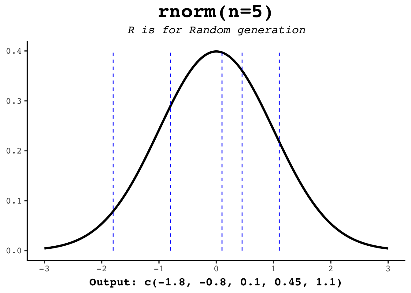

Figure 21.15: The rnorm function takes a number of samples and returns a vector of random numbers from the normal distribution (with mean=0, sd=1 as defaults)

21.7 Worked example: IQ scores

The normal distribution (also called the Gaussian distribution) is defined by two numbers: the mean (µ), which sets the centre, and the standard deviation (σ), which sets the spread. IQ scores are deliberately built to be normal with a mean of 100 and a standard deviation of 15, which makes them a perfect playground for the four functions.

A handy rule of thumb — the “68–95–99.7 rule” — says about 68% of values fall within one standard deviation of the mean (here, 85 to 115) and about 95% within two (70 to 130). Let’s check the 68% with pnorm. The area between 85 and 115 is the area below 115 minus the area below 85:

pnorm(115, mean = 100, sd = 15) - pnorm(85, mean = 100, sd = 15)

[1] 0.6826895

About 0.68 — exactly what the rule promises. Notice the pattern: a “between” question becomes one pnorm minus another.

21.8 Exercises

Use the IQ distribution (mean 100, sd 15) for each. Each solution names which of the four functions fits the question — that choice is the real skill.

Top 10%. Which IQ score marks the 90th percentile — the cutoff above which only the top 10% fall?
NoteSolution
qnorm(0.9, mean = 100, sd = 15)

[1] 119.2233
We want a value from a probability, so this is a qnorm job. About 119.
Above 130. What fraction of people have an IQ above 130 (two standard deviations up)?
NoteSolution
1 - pnorm(130, mean = 100, sd = 15)

[1] 0.02275013

# or, equivalently: pnorm(130, mean = 100, sd = 15, lower.tail = FALSE)

[1] 0.02275013
About 2.3% — consistent with the 95% rule leaving roughly 2.5% in each tail.
Below 70. What fraction have an IQ below 70?
NoteSolution
pnorm(70, mean = 100, sd = 15)

[1] 0.02275013
Also about 2.3%. The curve is symmetric, so the lower tail past 70 mirrors the upper tail past 130.
Simulate a classroom. Draw 30 random IQ scores and count how many land above
1. (Set a seed so your answer is reproducible.)
NoteSolution
set.seed(1) scores <- rnorm(30, mean = 100, sd = 15) sum(scores > 115)

[1] 3
Theory predicts about 16% above 115 — roughly 5 of 30 — but any single small sample wobbles around that. Re-run with a different seed to feel the sampling variability for yourself.

21.9 Summary

You now have the four-function toolkit for the normal distribution — and, thanks to R’s naming rule, the blueprint for every other distribution too:

pnorm(x) — area to the left of x (a probability). Use lower.tail = FALSE or 1 - pnorm(x) for the right tail, and one pnorm minus another for a range.
dnorm(x) — the height of the curve at x (a density).
qnorm(p) — the value at probability p (the inverse of pnorm); your tool for percentiles.
rnorm(n) — n random draws; pair it with set.seed() for reproducible simulations.

Keep the pictures in mind: pnorm is an area, dnorm is a height, qnorm reads the area axis backwards to a value, and rnorm scatters points along the curve.