29 Worked example: predicting gene expression from histone marks

Author

Affiliation

University of Colorado
Anschutz School of Medicine

Published

June 1, 2024

Modified

June 23, 2026

A gene’s DNA sequence doesn’t change from one cell type to the next, yet the same gene can be switched loudly on in one tissue and silent in another. Much of that control is written in histone modifications — chemical marks on the proteins that DNA wraps around, concentrated near each gene’s promoter. This example asks a question at the heart of gene regulation: can the pattern of histone modifications near a gene predict that gene’s expression level? (Figure 29.1)

This is the third of three worked examples, and like the methylation age example it is a regression problem — the target is a continuous expression level. We use the same mlr3 framework throughout; for the four building blocks see The mlr3verse, and for the general train/predict/assess workflow see the cancer example. Here the new idea is penalized regression with cross-validation, and a peek under the hood at how R² is actually computed.

This chapter views the same three ideas through the lens of regularization:

Feature selection, done automatically. In the cancer chapter you hand-picked features — you ranked genes by variance and kept the top 200. Penalized regression flips that around: instead of you choosing which features to drop, the model’s L1 (lasso) penalty shrinks the coefficients of useless features all the way to zero, selecting features for you as a side effect of fitting. Same goal — fewer, more useful features — but the work moves from your hands into the algorithm.
Cross-validation, inside the training set. A penalty has a strength, λ, and we have to choose it. The trick is to choose it by cross-validation within the training data — carving the training set into folds, never touching the test set. This is a fresh facet of the same golden rule from the cancer and methylation chapters: the test set stays sealed until the very end.
Overfitting, as a tunable knob. Regularization reframes overfitting as something you can dial. The penalty λ is a knob that trades a tighter fit on the training data for better generalization to new genes: turn it up and the model gets simpler and steadier; turn it down and it bends closer to the training points, at the risk of memorizing noise.

From a manual filter to an automatic penalty

The cancer chapter selected features by hand (keep the most variable genes); this chapter lets the model do it. A lasso penalty is, in effect, automatic feature selection baked into the fit — and cross-validation, run only on the training data, is how we pick how aggressive that penalty should be. The held-out test set is never consulted while we tune; it is saved for the single honest score at the end.

29.1 What you’ll learn

Center and scale features, and visualize them with boxplots and a heatmap.
Build a regression task and split it with mlr3’s partition() helper.
Fit penalized regression (ridge) with regr.cv_glmnet, and explain how cross-validation within the training set chooses the penalty strength λ.
Read a penalized model’s coefficients, contrast ridge with lasso, and see how the lasso penalty performs automatic feature selection — the job you did by hand in the cancer chapter.
Compute R² by hand and confirm it matches the regr.rsq measure.

29.2 Setup

library(mlr3verse)
library(mlr3learners) # for cv_glmnet
library(mlr3viz)      # for plotting predictions
library(ComplexHeatmap)
set.seed(789)

\[ y \sim h_1 + h_2 + h_3 + \ldots \tag{29.1}\]

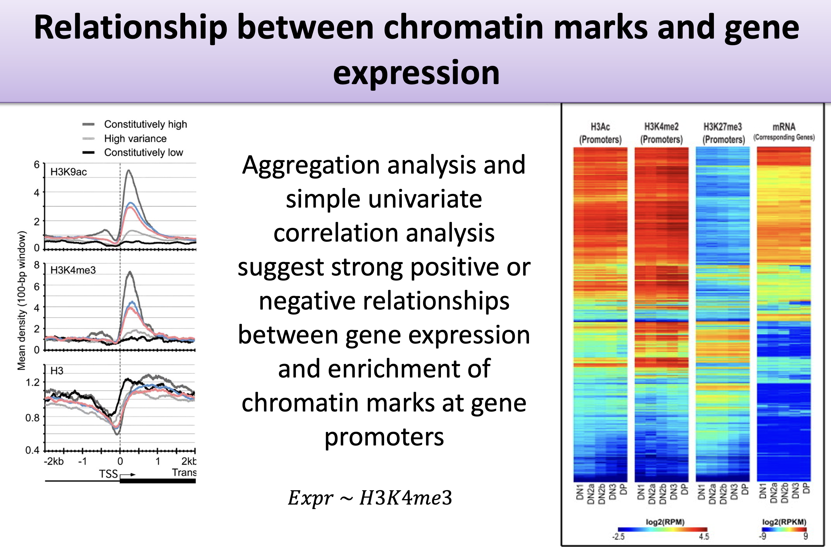
Figure 29.1: What is the combined effect of histone marks on gene expression?

The data summarize the histone marks within each gene’s promoter (here, the region 2 kb upstream of the transcription start site), paired with that gene’s measured expression. The target is the expression level; the features are the histone-mark summaries. As Equation 29.1 sketches, we are modelling expression $y$ as a combination of histone marks $h_1, h_2, \ldots$. We’ll try two approaches: penalized regression and a random forest.

29.3 The data

The data were developed by Anshul Kundaje. We won’t dwell on the collection details; we’ll focus on the modelling.

feature_set <- read.table("http://seandavi.github.io/ITR/expression-prediction/features.txt")

What are the predictor columns?

colnames(feature_set)

 [1] "Control"  "Dnase"    "H2az"     "H3k27ac"  "H3k27me3" "H3k36me3"
 [7] "H3k4me1"  "H3k4me2"  "H3k4me3"  "H3k79me2" "H3k9ac"   "H3k9me1" 
[13] "H3k9me3"  "H4k20me1"

These histone-mark summaries are our predictors. Some learners assume the predictors are on a similar scale, so we center and scale each column (subtract its mean, divide by its standard deviation) by converting to a matrix and using scale().

par(mfrow = c(1, 2))
scaled_features <- scale(as.matrix(feature_set))
boxplot(feature_set, main = 'Original data')
boxplot(scaled_features, main = 'Centered and scaled data')

Figure 29.2: Boxplots of the original and the centered-and-scaled features. After scaling, every feature sits on a comparable scale.

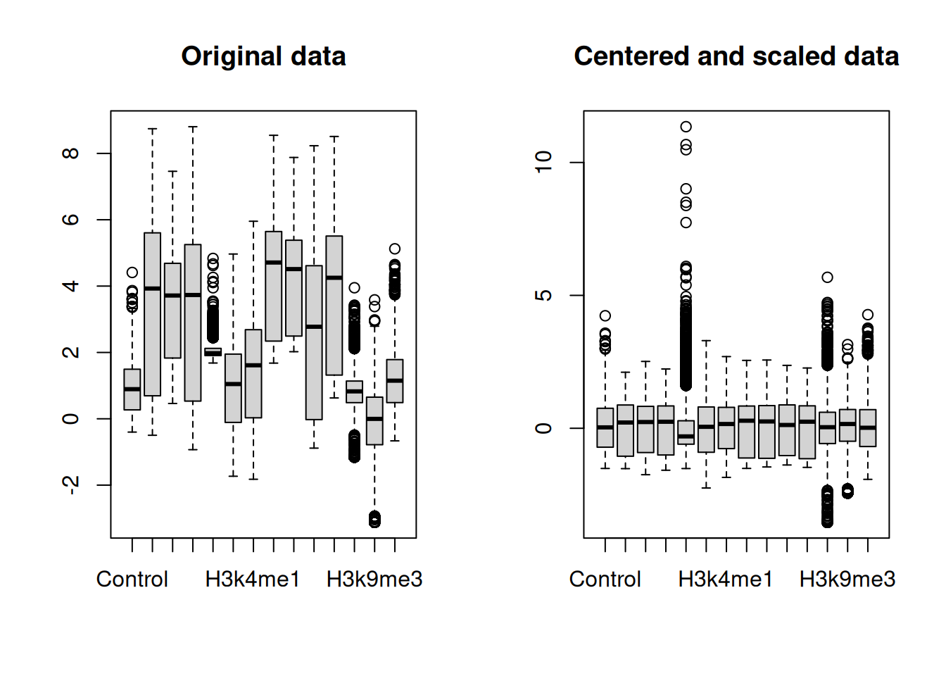
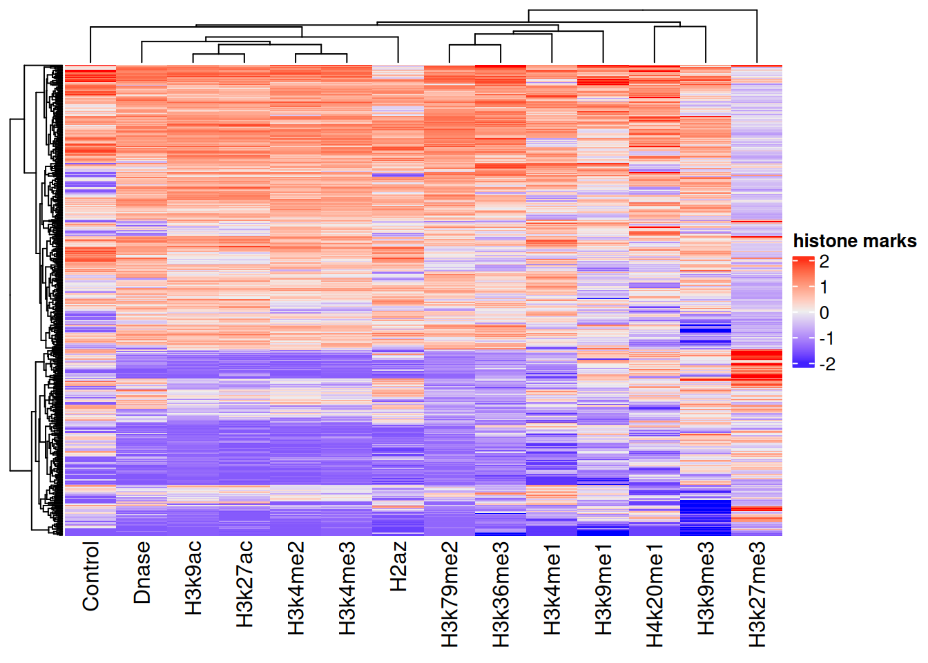
After scaling, every feature is centered near zero with comparable spread, as the right-hand boxplot shows. We can also spot structure across genes with a heatmap (Figure 29.3).

set.seed(789)
sampled_features <- scaled_features[sample(nrow(scaled_features), 500), ]
Heatmap(sampled_features, name = 'histone marks', show_row_names = FALSE)

Figure 29.3: Heatmap of 500 randomly sampled genes (rows) across the histone marks (columns). Blocks of similar color reveal groups of genes with similar mark patterns.

Now we read in the matching gene-expression values — our prediction target — and combine them with the scaled features into one data frame.

target <- scan(url("http://seandavi.github.io/ITR/expression-prediction/target.txt"), skip = 1)
# combine target and features into one data frame
exp_pred_data <- data.frame(gene_expression = target, scaled_features)

The first few rows:

head(exp_pred_data, 3)

                            gene_expression    Control      Dnase       H2az
ENSG00000000419.7.49575069         6.082343  0.7452926  0.7575546  1.0728432
ENSG00000000457.8.169863093        2.989145  1.9509786  1.0216546  0.3702787
ENSG00000000938.7.27961645        -5.058894 -0.3505542 -1.4482958 -1.0390775
                               H3k27ac   H3k27me3   H3k36me3    H3k4me1
ENSG00000000419.7.49575069   1.0950440 -0.5125312  1.1334793  0.4127984
ENSG00000000457.8.169863093  0.7142157 -0.4079244  0.8739005  1.1649282
ENSG00000000938.7.27961645  -1.0173283  1.4117293 -0.5157582 -0.5017450
                               H3k4me2    H3k4me3   H3k79me2     H3k9ac
ENSG00000000419.7.49575069   1.2136176  1.1202901  1.5155803  1.2468256
ENSG00000000457.8.169863093  0.6456572  0.6508561  0.7976487  0.5792891
ENSG00000000938.7.27961645  -0.1878255 -0.6560973 -1.3803974 -1.0067972
                              H3k9me1   H3k9me3   H4k20me1
ENSG00000000419.7.49575069  0.1426980  1.185622  1.9599992
ENSG00000000457.8.169863093 0.3630902  1.014923 -0.2695111
ENSG00000000938.7.27961645  0.6564520 -1.370871 -1.8773178

29.4 Create the task and split

The target is a number, so this is a regression task. This time we use mlr3’s own partition() helper to make the train/test split, which by default holds out one-third for testing.

set.seed(7)
exp_pred_task <- as_task_regr(exp_pred_data, target = 'gene_expression')
split <- partition(exp_pred_task)

29.5 Linear regression

As a baseline, fit an ordinary linear regression.

learner <- lrn("regr.lm")

29.5.1 Train and predict

learner$train(exp_pred_task, split$train)
pred_train <- learner$predict(exp_pred_task, split$train)
pred_test <- learner$predict(exp_pred_task, split$test)

29.5.2 Assess

pred_train


── <PredictionRegr> for 5789 observations: ─────────────────────────────────────
 row_ids     truth  response
       2  2.989145  2.996674
       3 -5.058894 -5.364407
       5  5.558023  4.105793
     ---       ---       ---
    8639 -5.058894 -5.238131
    8640 -3.114148 -4.756313
    8641  5.731075  4.198905

plot(pred_train)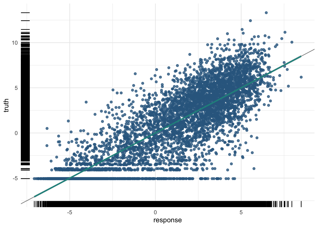

Figure 29.4: Linear-regression predictions on the **training** genes: predicted expression (vertical) against measured expression (horizontal), one point per gene. The closer the points cluster along the diagonal, the more of the expression signal the histone marks are capturing.

The training R²:

measures <- msrs(c('regr.rsq'))
pred_train$score(measures)

 regr.rsq 
0.7507266

And the test R² — the number that matters:

pred_test$score(measures)

 regr.rsq 
0.7505519

plot(pred_test)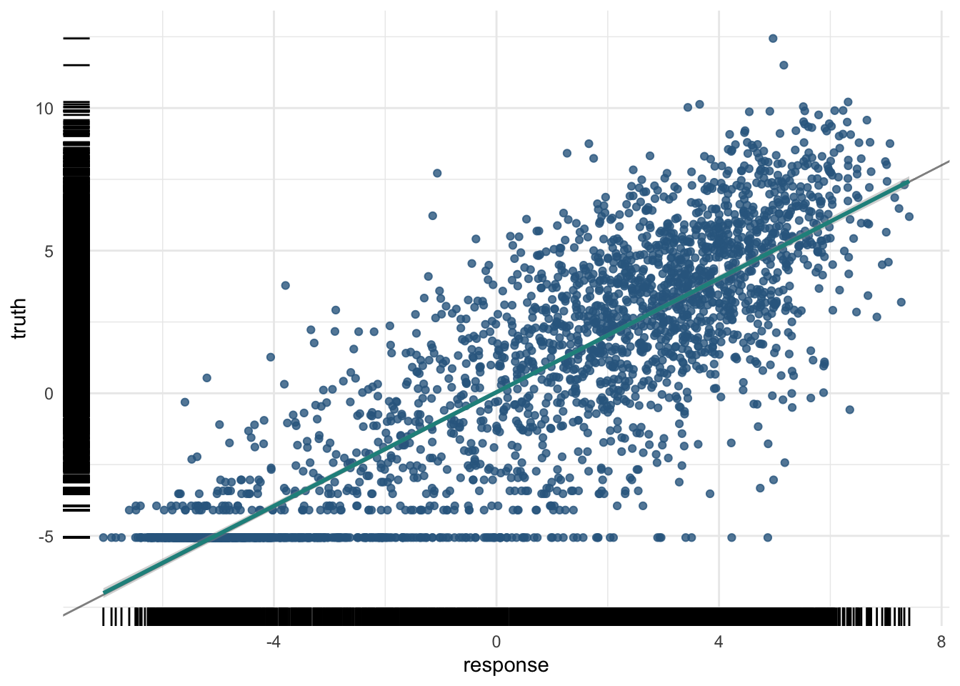

Figure 29.5: Linear-regression predictions on the held-out **test** genes. Because the model never saw these genes during training, this scatter is the honest picture of how well promoter histone marks predict a gene’s expression.

A moderate R² here is a real biological result: histone marks in the promoter carry genuine, but partial, information about how strongly a gene is expressed.

29.6 Penalized regression

When a model has many predictors, it can become too flexible and start fitting noise — the problem of overfitting. Penalized regression combats this by adding a penalty for complexity, nudging the model toward simpler, more general solutions.

Three flavours of penalty

Ridge (L2): shrinks all coefficients toward zero, like a rubber band pulling them in. It keeps every feature but tames large coefficients.
Lasso (L1): can shrink some coefficients all the way to zero, like scissors that cut the least useful features out of the model entirely. This doubles as automatic feature selection.
Elastic net: a blend of the two — rubber band and scissors — combining shrinkage with feature elimination.

In mlr3, the alpha setting picks the flavour: alpha = 0 is ridge, alpha = 1 is lasso, and values in between are elastic net.

Whichever flavour you pick, a single dial controls how hard the penalty pushes: the regularization strength λ (lambda). At λ = 0 there is no penalty at all and you are back to ordinary least squares — the most flexible, highest-variance fit. Turn λ up and the coefficients are squeezed toward zero, giving a simpler, higher-bias model. In other words, λ is a knob that slides the model back and forth along the model-complexity axis from the introduction (Figure 29.6). The whole game is to stop at the bottom of the U — and that is exactly the job we hand to cross-validation.

Code

library(ggplot2)
x        <- seq(0, 10, length.out = 400)
bias2    <- exp(-0.5 * x)
variance <- 0.01 * exp(0.5 * x)
total    <- bias2 + variance + 0.12
opt      <- x[which.min(total)]
df <- data.frame(
  x     = rep(x, 3),
  error = c(total, variance, bias2),
  curve = factor(rep(c("Total error", "Variance", "Bias²"), each = length(x)),
                 levels = c("Total error", "Variance", "Bias²")))
cols <- c("Total error" = "#1a1a1a", "Variance" = "#3a9aa5", "Bias²" = "#a8322a")
ggplot(df, aes(x, error, colour = curve)) +
  annotate("segment", x = 0, xend = 0, y = 0, yend = 1.72,
           arrow = arrow(length = unit(0.22, "cm"), type = "closed"), linewidth = 0.5) +
  annotate("segment", x = 0, xend = 10.7, y = 0, yend = 0,
           arrow = arrow(length = unit(0.22, "cm"), type = "closed"), linewidth = 0.5) +
  annotate("segment", x = opt, xend = opt, y = 0, yend = 1.5,
           linetype = "dotted", colour = "grey25", linewidth = 0.5) +
  annotate("text", x = opt - 0.18, y = 1.0, label = "λ chosen by cross-validation",
           angle = 90, fontface = "italic", size = 3.1, colour = "grey20") +
  geom_line(linewidth = 1.1) +
  annotate("text", x = 6.1, y = 1.34, label = "Total error", colour = cols[["Total error"]], size = 3.8) +
  annotate("text", x = 8.9, y = 0.78, label = "Variance",    colour = cols[["Variance"]],    size = 3.8) +
  annotate("text", x = 8.9, y = 0.14, label = "Bias²",  colour = cols[["Bias²"]],  size = 3.8) +
  annotate("text", x = 5.3, y = -0.12, label = "Model complexity", size = 3.6) +
  # the lambda dial beneath the axis
  annotate("segment", x = 9.3, xend = 1.0, y = -0.34, yend = -0.34,
           arrow = arrow(length = unit(0.22, "cm"), type = "closed"),
           colour = "#3b6ea5", linewidth = 0.7) +
  annotate("text", x = 9.95, y = -0.34, label = "λ = 0\n(OLS)", hjust = 0,
           size = 2.9, colour = "grey20", lineheight = 0.85) +
  annotate("text", x = 0.55, y = -0.34, label = "large λ", hjust = 1,
           size = 2.9, colour = "grey20") +
  annotate("text", x = 5.2, y = -0.52,
           label = "increasing λ  (stronger penalty → simpler model)",
           colour = "#3b6ea5", size = 3.3) +
  scale_colour_manual(values = cols) +
  scale_x_continuous(expand = c(0, 0)) +
  scale_y_continuous(expand = c(0, 0)) +
  coord_cartesian(xlim = c(-0.7, 11.4), ylim = c(-0.62, 1.82), clip = "off") +
  annotate("text", x = -0.5, y = 0.85, label = "Error", angle = 90, size = 4) +
  theme_void() +
  theme(legend.position = "none", plot.margin = margin(6, 14, 10, 18))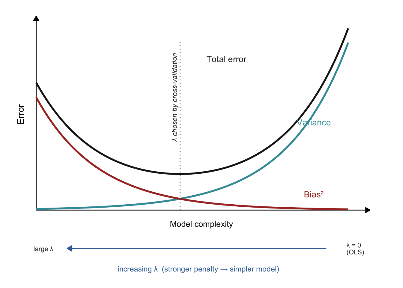

Figure 29.6: Penalized regression turns model complexity into a single continuous dial. The curves are the same bias–variance picture from the introduction: as the model grows more complex, **bias²** falls while **variance** rises, and their sum — the **total error** on new data — traces a U. What penalized regression adds is the λ knob along the bottom. At **λ = 0** there is no penalty and you fit ordinary least squares: the most complex, highest-variance model (far right). Increasing λ shrinks the coefficients, sliding the model leftward toward simpler, higher-bias fits. Cross-validation’s one job is to find the λ that lands at the bottom of the U.

We’ll use the regr.cv_glmnet learner, which automatically uses cross-validation to choose the penalty strength.

What is cross-validation?

Cross-validation estimates how a model will perform on unseen data by splitting the training data into k equal folds. The model trains on k − 1 folds and is validated on the held-out fold, repeating until each fold has served as the validation set once. Averaging the k scores gives a stable performance estimate, and cv_glmnet uses it to pick the best penalty (lambda). The nfolds setting controls k; 5 or 10 are common choices.

Here is how that actually pins down the penalty. cv_glmnet lays out a grid of candidate λ values, from strong to weak. For each candidate it runs the full k-fold routine just described — fit on k − 1 folds, measure the error on the held-out fold, rotate until every fold has taken a turn as validation set — and averages those k errors into a single score for that λ. Sweeping across the whole grid therefore yields one cross-validated error per candidate penalty (the curve we plot in a moment). The best λ is then simply the one with the lowest cross-validated error — glmnet calls it lambda.min. Because that minimum can be a little noisy, glmnet also offers lambda.1se: the strongest penalty (the simplest model) whose error is still within one standard error of the best, a slightly more conservative default. The essential point is that this entire search happens inside the training data — the test set is never consulted while we choose λ, so it remains a fair, untouched judge at the end.

With alpha = 0 we fit a ridge model with 10-fold cross-validation:

set.seed(789)
learner <- lrn("regr.cv_glmnet", nfolds = 10, alpha = 0)

29.6.1 Train

learner$train(exp_pred_task, split$train)

Because cv_glmnet quietly tried a whole range of λ values and scored each one by cross-validation, we can look at that search directly (Figure 29.7) — the real-data version of the λ dial from the schematic above.

plot(learner$model)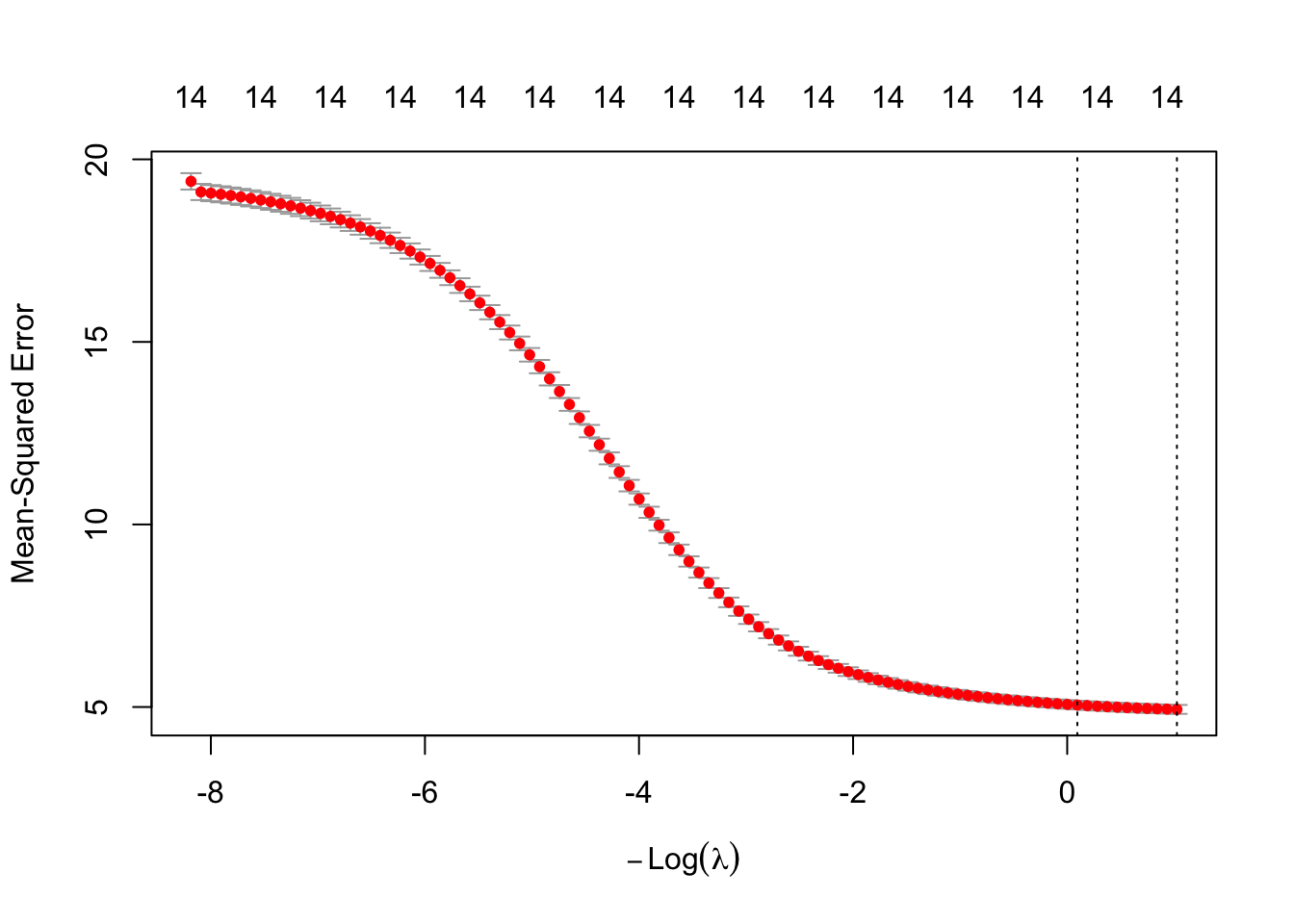

Figure 29.7: The cross-validation search that `cv_glmnet` ran. Each red dot is the mean cross-validated error (mean squared error) for one value of the penalty, with vertical bars showing ±1 standard error; the numbers across the top count how many features survive at each λ — all 14 here, because *ridge* shrinks coefficients but never zeros them (only lasso would prune that count). The x-axis is **−log(λ)**, so the penalty grows toward the *left*, the same orientation as the schematic above. The two dotted lines mark **lambda.min** (lowest CV error) and **lambda.1se** (the strongest penalty within one standard error of it). Notice the error keeps falling as the penalty weakens, with no interior bottom: on this small, low-dimensional dataset ridge’s shrinkage buys little, and cross-validation settles near the lightly-penalized, OLS-like end. Penalties earn their keep when features are many and correlated — not so much here.

For a penalized model we can inspect the coefficients directly:

coef(learner$model)

15 x 1 sparse Matrix of class "dgCMatrix"
             lambda.1se
(Intercept)  0.08832251
Control     -0.05020310
Dnase        0.85954551
H2az         0.31828260
H3k27ac      0.26566165
H3k27me3    -0.27170626
H3k36me3     0.65845540
H3k4me1     -0.02832563
H3k4me2      0.17902035
H3k4me3      0.37064260
H3k79me2     0.86371398
H3k9ac       0.48125738
H3k9me1     -0.05440077
H3k9me3     -0.16204169
H4k20me1     0.13611422

Each coefficient tells us how strongly its histone mark pushes predicted expression up or down. With lasso (alpha = 1) many of these would be exactly zero — the model would have selected a subset of marks for us, which is useful not just for prediction but for understanding which marks matter.

Cross-validation tunes the model; the test set still judges it

It is tempting to think that once you have cross-validated, you are done — but the two jobs are different, and they deliberately use different data. The cross-validation inside cv_glmnet ran entirely on the training split (split$train): it carved those training genes into 10 folds to choose λ, and never touched split$test. That makes it a tuning tool, not an honest performance estimate — the chosen λ has, in effect, been fitted to the training data, so scoring the model on that same data would flatter it.

This is exactly why we set aside a test set with partition() at the very start. We still report the model’s quality on the held-out test genes below (split$test), which played no part in fitting the coefficients or in selecting λ. Cross-validation picks the dial; the untouched test set delivers the verdict.

29.6.2 Predict and assess

pred_train <- learner$predict(exp_pred_task, split$train)
pred_test <- learner$predict(exp_pred_task, split$test)

pred_train


── <PredictionRegr> for 5789 observations: ─────────────────────────────────────
 row_ids     truth  response
       2  2.989145  2.933043
       3 -5.058894 -4.471610
       5  5.558023  4.221675
     ---       ---       ---
    8639 -5.058894 -5.581904
    8640 -3.114148 -4.105914
    8641  5.731075  4.427548

plot(pred_train)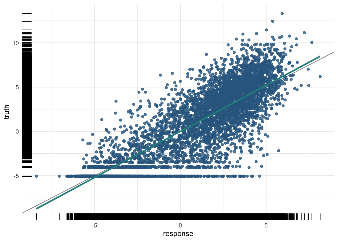

Figure 29.8: Ridge-regression predictions on the **training** genes. The L2 penalty shrinks the coefficients to curb overfitting, so the training fit may look slightly looser than plain linear regression — the payoff is steadier predictions on new genes.

The training R²:

measures <- msrs(c('regr.rsq'))
pred_train$score(measures)

regr.rsq 
0.740439

And the test R²:

pred_test$score(measures)

 regr.rsq 
0.7405317

plot(pred_test)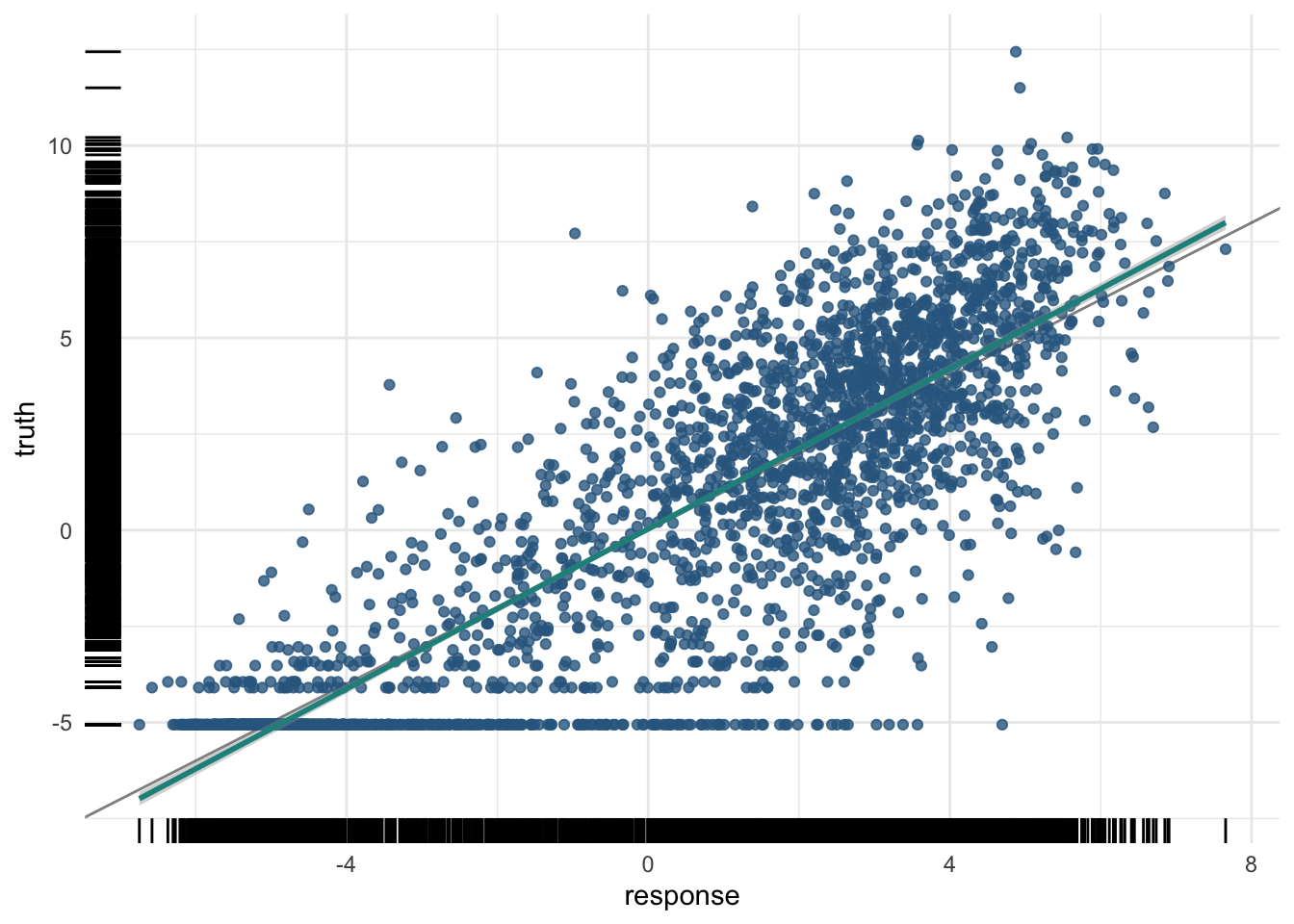

Figure 29.9: Ridge-regression predictions on the held-out **test** genes — the honest comparison against the linear model above. With only a handful of histone-mark features here, ridge and plain linear regression land in a similar place; the penalty earns its keep when features are many and correlated.

We can also compute the test R² by hand, to demystify the measure: it is one minus the ratio of the residual sum of squares to the total sum of squares.

# calculate the R-squared value by hand
truth <- pred_test$truth
predicted <- pred_test$response
rss <- sum((truth - predicted)^2)          # residual sum of squares
tss <- sum((truth - mean(truth))^2)        # total sum of squares
r_squared <- 1 - (rss / tss)
r_squared

[1] 0.7405317

This matches the regr.rsq measure above — reassuring confirmation that you understand exactly what R² is counting.

29.7 Summary

You have now used machine learning to probe a question in gene regulation — whether promoter histone marks predict expression — through the same mlr3 workflow as the previous two chapters:

You scaled the histone-mark features, visualized them with boxplots and a heatmap, and built a regression task split with partition().
A baseline linear regression gave a moderate R² — a real, if partial, biological signal that marks carry information about expression.
Penalized regression (ridge via regr.cv_glmnet) used cross-validation to choose its penalty and fight overfitting; with lasso it would also perform feature selection, turning the model into a tool for understanding which marks matter.
Computing R² by hand confirmed exactly what the regr.rsq measure counts.

Across all three worked examples the same disciplines recurred: split the data, select features thoughtfully, train then predict, and judge every model by its test-set score. That last habit — never trusting the training score — is the single most important thing to carry forward.

29.8 Exercises

Each exercise reuses objects you already built, so the solutions are quick to run.

Change the number of CV folds. The ridge model used nfolds = 10. Refit it with nfolds = 5 and see whether the test R² changes much.
NoteSolution
ridge5 <- lrn("regr.cv_glmnet", nfolds = 5, alpha = 0) ridge5$train(exp_pred_task, split$train) ridge5$predict(exp_pred_task, split$test)$score(msrs(c('regr.rsq')))
Fewer folds means each training fold is a little smaller and the chosen penalty is a little noisier, but the test R² usually shifts only slightly. The penalty selection is fairly robust to the exact number of folds.
Try lasso instead of ridge. We used alpha = 0 (ridge). Refit with alpha = 1 (lasso) and inspect the coefficients. How many histone marks does lasso drop to exactly zero?
NoteSolution
lasso <- lrn("regr.cv_glmnet", nfolds = 10, alpha = 1) lasso$train(exp_pred_task, split$train) coef(lasso$model) # zeros are the dropped marks lasso$predict(exp_pred_task, split$test)$score(msrs(c('regr.rsq')))
Lasso sets the coefficients of the least useful marks to exactly zero, so the non-zero entries are the marks it “selected.” This is feature selection built into the model, and it makes the result easier to interpret biologically.
Add a random forest. The chapter opening promised a random forest too. Fit regr.ranger on the same task and split, and compare its test R² to ridge.
NoteSolution
rf <- lrn("regr.ranger") rf$train(exp_pred_task, split$train) rf$predict(exp_pred_task, split$test)$score(msrs(c('regr.rsq')))
Swapping the learner is a one-line change to lrn(). The forest can capture non-linear interactions between marks that a linear model cannot, so it sometimes edges out ridge — but, as always, the honest comparison is the held-out test R².