30 Working with a SummarizedExperiment
An RNA-seq or microarray experiment hands you several things at once: a matrix of numbers (counts or intensities), a description of every feature down the side (which gene is in each row), and a description of every sample across the top (which condition, which patient). Keep these in three separate variables and they will drift out of sync — you drop a bad sample from the count matrix, forget to drop it from the sample table, and now your “treated vs. control” labels point at the wrong columns. Mismatches exactly like this have produced retracted papers.
SummarizedExperiment is Bioconductor’s answer: one object that holds the assay matrix, the feature data, and the sample data together, and keeps them aligned for you whenever you subset. Almost every Bioconductor analysis package expects data in this shape, so learning to work with one — inspect it, reach into its parts, subset it, and plot from it — is the single most transferable skill in the Bioconductor half of this book.
This chapter is about using a SummarizedExperiment someone has handed you. The next chapter shows you how to build one from raw parts and share it.
30.1 What you’ll learn
By the end of this chapter you will be able to:
- Explain why a
SummarizedExperimentbeats juggling a matrix and two separate tables — and show the bug it prevents. - Map the
data.frameoperations you already know onto theirSummarizedExperimentequivalents. - Describe the three coordinated parts:
assays(),rowData(), andcolData(), plus experiment-widemetadata(). - Subset an experiment several different ways — by position, by sample phenotype, by a feature property, by feature annotation, and by name — and trust that the metadata follows.
- Select the most variable genes and draw an annotated heatmap whose sample labels come straight from
colData.
The examples below use the SummarizedExperiment class, the airway example dataset, and a couple of plotting helpers. Install them once with BiocManager:
30.2 Why not just a data frame?
You already know data frames. Why learn a new container at all? Because a single data frame can hold features down the side or sample information across the top, but not both at once. To keep a real experiment you’d end up with two or three loose objects and a promise to yourself to keep them lined up. That promise is exactly what breaks.
Watch it break. Here is a tiny experiment as loose pieces — a counts matrix and a separate sample table:
      S1 S2 S3
GeneA 10 30 50
GeneB 20 40 60
samples id group
1 S1 control
2 S2 control
3 S3 treatedSample S2 turns out to be bad, so you drop it from the counts matrix — but, in the rush, forget the sample table:
counts <- counts[, c("S1", "S3")]   # S2 removed here...
# ...but `samples` still has all three rows
counts
S1 S3
GeneA 10 50
GeneB 20 60samples id group
1 S1 control
2 S2 control
3 S3 treatedNothing errors. R has no idea these two objects are supposed to correspond. But now column 2 of counts is S3 (treated), while row 2 of samples still says S2 (control). Any analysis that reads “group” from samples and “numbers” from counts is now silently wrong. This is the class of mistake that retracts papers, and it is invisible — no warning, no red text.
A SummarizedExperiment removes the promise. The three pieces live in one object, and a single subsetting operation updates all of them together. There is no second table to forget.
You stop subsetting the matrix. You subset the object. Everything else — sample labels, feature annotation, every extra assay — follows automatically.
30.2.1 A data.frame → SummarizedExperiment Rosetta table
Most of what you know transfers directly; only the vocabulary changes.
| What you want | data.frame |
SummarizedExperiment (se) |
|---|---|---|
| Dimensions | dim(df) |
dim(se) (features × samples) |
| Row / column count |
nrow(df), ncol(df)
|
nrow(se), ncol(se)
|
| Names |
rownames(df), colnames(df)
|
rownames(se), colnames(se)
|
| A rectangular slice | df[rows, cols] |
se[features, samples] |
| The numbers | the columns themselves |
assay(se) / assays(se)
|
| A piece of sample info | df$group |
se$group (reaches colData) |
| A piece of feature info | — | rowData(se)$symbol |
| Filter by a sample property | df[df$group == "treated", ] |
se[, se$group == "treated"] |
$ gotcha
On a data frame, df$x pulls out a column of data. On a SummarizedExperiment, se$x pulls out a column of sample metadata (colData) — not a column of the assay. It is the single most common point of confusion. The numbers live in assay(se); $ is for sample annotation.
30.3 Anatomy of a SummarizedExperiment
A SummarizedExperiment is a matrix-like container where rows represent features of interest (e.g. genes, transcripts, exons) and columns represent samples. The object holds one or more assays, each a matrix-like object of numeric (or other) values. Information about the features is stored in a DataFrame accessible with rowData(); each of its rows describes the feature in the corresponding row of the object, and its columns are feature attributes (gene IDs, symbols, biotypes, and so on). Sample information lives in a parallel DataFrame reached with colData().
Figure 30.1 shows the class geometry and the vertical (column) and horizontal (row) relationships.
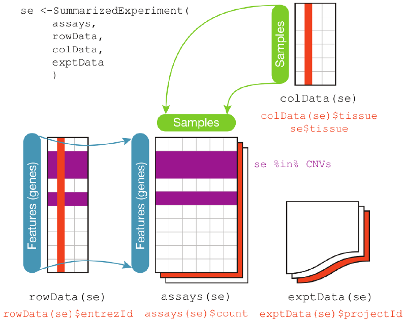
SummarizedExperiment has three main components: the colData(), the rowData(), and the assays(). The accessors for each part share its name. Figure from the Bioconductor SummarizedExperiment vignette (Morgan, Obenchain, Hester & Pagès; Artistic-2.0).
Picture a spreadsheet workbook with three sheets that are locked together:
- the assay sheet — the matrix of numbers, features (genes) × samples;
- the row sheet (
rowData) — one row of annotation per feature, lined up with the assay’s rows; - the column sheet (
colData) — one row of annotation per sample, lined up with the assay’s columns.
The magic is the lock: when you delete a sample, all three sheets update together, so the numbers and their labels can never disagree. Every accessor below is just a way of looking at one of these sheets.
Loading required package: airwayWe’ll use the airway dataset: an RNA-seq experiment of read counts per gene for airway smooth muscle cells, across 8 samples. It actually ships as a RangedSummarizedExperiment — its rows carry genomic coordinates — but we’ll set that aside and coerce it to a plain SummarizedExperiment, so the row information is a simple annotation table:
library(SummarizedExperiment)
data(airway, package="airway")
se <- as(airway, "SummarizedExperiment")
se
class: SummarizedExperiment
dim: 63677 8
metadata(1): ''
assays(1): counts
rownames(63677): ENSG00000000003 ENSG00000000005 ... ENSG00000273492
ENSG00000273493
rowData names(10): gene_id gene_name ... seq_coord_system symbol
colnames(8): SRR1039508 SRR1039509 ... SRR1039520 SRR1039521
colData names(9): SampleName cell ... Sample BioSampleRead that printout like a label on the box: dim tells you it’s 63,677 features across 8 samples, and the assays, rowData, and colData lines preview the three linked sheets. The next sections open each one in turn.
RangedSummarizedExperiment
When features are genes, exons, or peaks, they sit at positions on the genome. A sibling class, RangedSummarizedExperiment, stores those positions as a GRanges/GRangesList reachable with rowRanges() (in place of rowData()), which unlocks genomic operations like subsetByOverlaps(). The airway data is really one of these — we coerced it to a plain SummarizedExperiment above to keep the focus on the core idea. Once you’ve met GRanges in the genomic-ranges chapters, come back: airway’s ranges will be waiting, and everything you learn here still applies.
30.3.1 Assays — the numbers
Retrieve the experiment data with the assays() accessor. An object can hold multiple assays, each reachable by name with $. The airway dataset has a single assay, counts, where each row is a gene and each column a sample.
assays(se)$counts| SRR1039508 | SRR1039509 | SRR1039512 | SRR1039513 | SRR1039516 | SRR1039517 | SRR1039520 | SRR1039521 | |
|---|---|---|---|---|---|---|---|---|
| ENSG00000000003 | 679 | 448 | 873 | 408 | 1138 | 1047 | 770 | 572 |
| ENSG00000000005 | 0 | 0 | 0 | 0 | 0 | 0 | 0 | 0 |
| ENSG00000000419 | 467 | 515 | 621 | 365 | 587 | 799 | 417 | 508 |
| ENSG00000000457 | 260 | 211 | 263 | 164 | 245 | 331 | 233 | 229 |
| ENSG00000000460 | 60 | 55 | 40 | 35 | 78 | 63 | 76 | 60 |
| ENSG00000000938 | 0 | 0 | 2 | 0 | 1 | 0 | 0 | 0 |
| ENSG00000000971 | 3251 | 3679 | 6177 | 4252 | 6721 | 11027 | 5176 | 7995 |
| ENSG00000001036 | 1433 | 1062 | 1733 | 881 | 1424 | 1439 | 1359 | 1109 |
| ENSG00000001084 | 519 | 380 | 595 | 493 | 820 | 714 | 696 | 704 |
| ENSG00000001167 | 394 | 236 | 464 | 175 | 658 | 584 | 360 | 269 |
30.3.2 Row data — what each feature is
rowData() returns a DataFrame with one row per feature, lined up with the assay’s rows. For airway, each gene arrives annotated with its Ensembl ID, gene symbol, biotype, and more — a table you can read and filter like any other:
rowData(se)DataFrame with 63677 rows and 10 columns
gene_id gene_name entrezid gene_biotype
<character> <character> <integer> <character>
ENSG00000000003 ENSG00000000003 TSPAN6 NA protein_coding
ENSG00000000005 ENSG00000000005 TNMD NA protein_coding
ENSG00000000419 ENSG00000000419 DPM1 NA protein_coding
ENSG00000000457 ENSG00000000457 SCYL3 NA protein_coding
ENSG00000000460 ENSG00000000460 C1orf112 NA protein_coding
... ... ... ... ...
ENSG00000273489 ENSG00000273489 RP11-180C16.1 NA antisense
ENSG00000273490 ENSG00000273490 TSEN34 NA protein_coding
ENSG00000273491 ENSG00000273491 RP11-138A9.2 NA lincRNA
ENSG00000273492 ENSG00000273492 AP000230.1 NA lincRNA
ENSG00000273493 ENSG00000273493 RP11-80H18.4 NA lincRNA
gene_seq_start gene_seq_end seq_name seq_strand
<integer> <integer> <character> <integer>
ENSG00000000003 99883667 99894988 X -1
ENSG00000000005 99839799 99854882 X 1
ENSG00000000419 49551404 49575092 20 -1
ENSG00000000457 169818772 169863408 1 -1
ENSG00000000460 169631245 169823221 1 1
... ... ... ... ...
ENSG00000273489 131178723 131182453 7 -1
ENSG00000273490 54693789 54697585 HSCHR19LRC_LRC_J_CTG1 1
ENSG00000273491 130600118 130603315 HG1308_PATCH 1
ENSG00000273492 27543189 27589700 21 1
ENSG00000273493 58315692 58315845 3 1
seq_coord_system symbol
<integer> <character>
ENSG00000000003 NA TSPAN6
ENSG00000000005 NA TNMD
ENSG00000000419 NA DPM1
ENSG00000000457 NA SCYL3
ENSG00000000460 NA C1orf112
... ... ...
ENSG00000273489 NA RP11-180C16.1
ENSG00000273490 NA TSEN34
ENSG00000273491 NA RP11-138A9.2
ENSG00000273492 NA AP000230.1
ENSG00000273493 NA RP11-80H18.430.3.3 Column data — what each sample is
Sample metadata lives in colData(), a DataFrame with one row per sample and as many descriptive columns as you like.
colData(se)DataFrame with 8 rows and 9 columns
SampleName cell dex albut Run avgLength
<factor> <factor> <factor> <factor> <factor> <integer>
SRR1039508 GSM1275862 N61311 untrt untrt SRR1039508 126
SRR1039509 GSM1275863 N61311 trt untrt SRR1039509 126
SRR1039512 GSM1275866 N052611 untrt untrt SRR1039512 126
SRR1039513 GSM1275867 N052611 trt untrt SRR1039513 87
SRR1039516 GSM1275870 N080611 untrt untrt SRR1039516 120
SRR1039517 GSM1275871 N080611 trt untrt SRR1039517 126
SRR1039520 GSM1275874 N061011 untrt untrt SRR1039520 101
SRR1039521 GSM1275875 N061011 trt untrt SRR1039521 98
Experiment Sample BioSample
<factor> <factor> <factor>
SRR1039508 SRX384345 SRS508568 SAMN02422669
SRR1039509 SRX384346 SRS508567 SAMN02422675
SRR1039512 SRX384349 SRS508571 SAMN02422678
SRR1039513 SRX384350 SRS508572 SAMN02422670
SRR1039516 SRX384353 SRS508575 SAMN02422682
SRR1039517 SRX384354 SRS508576 SAMN02422673
SRR1039520 SRX384357 SRS508579 SAMN02422683
SRR1039521 SRX384358 SRS508580 SAMN02422677Each row is one sample; each column is something we know about it — including dex, whether the cells were treated with dexamethasone. That dex column is what makes phenotype-based subsetting possible, and it is what we’ll annotate the heatmap with later.
30.3.4 Experiment-wide metadata
Information about the experiment as a whole — methods, references, anything you like — lives in metadata(), which is just a plain list.
metadata(se)[[1]]
Experiment data
Experimenter name: Himes BE
Laboratory: NA
Contact information:
Title: RNA-Seq transcriptome profiling identifies CRISPLD2 as a glucocorticoid responsive gene that modulates cytokine function in airway smooth muscle cells.
URL: http://www.ncbi.nlm.nih.gov/pubmed/24926665
PMIDs: 24926665
Abstract: A 226 word abstract is available. Use 'abstract' method.Because it’s an ordinary list, you can stash anything in it, such as the model formula you intend to use downstream:
metadata(se)$formula <- counts ~ cell + dex
metadata(se)
[[1]]
Experiment data
Experimenter name: Himes BE
Laboratory: NA
Contact information:
Title: RNA-Seq transcriptome profiling identifies CRISPLD2 as a glucocorticoid responsive gene that modulates cytokine function in airway smooth muscle cells.
URL: http://www.ncbi.nlm.nih.gov/pubmed/24926665
PMIDs: 24926665
Abstract: A 226 word abstract is available. Use 'abstract' method.
$formula
counts ~ cell + dexcounts ~ cell + dex is an R formula — a compact way to say “the thing on the left is modeled by the things on the right.” The ~ reads as “is explained by” (or simply “by”), and + adds terms. So this one says “model the counts using both the cell line and the treatment.” Formulas are how you specify models all over R: t.test(), lm(), ggplot2’s facet_*(), and differential-expression tools like DESeq2 all take one. Here we are only storing the formula as a note — nothing is fitted yet. We wrote ~ cell + dex (rather than ~ dex alone) for a concrete reason you’ll see in the heatmap below: the donor (cell) is a big source of variation, so a sensible model accounts for it alongside the treatment.
30.4 A subsetting cookbook
Every example below subsets the object and lets the metadata follow. That is the whole point — you never maintain a second table by hand.
By position, exactly like a matrix ([features, samples]):
se[1:5, 1:3] # first five genes, first three samplesclass: SummarizedExperiment
dim: 5 3
metadata(2): '' formula
assays(1): counts
rownames(5): ENSG00000000003 ENSG00000000005 ENSG00000000419
ENSG00000000457 ENSG00000000460
rowData names(10): gene_id gene_name ... seq_coord_system symbol
colnames(3): SRR1039508 SRR1039509 SRR1039512
colData names(9): SampleName cell ... Sample BioSampleBy sample phenotype, using $ on colData:
se[, se$dex == "trt"] # only dexamethasone-treated samplesclass: SummarizedExperiment
dim: 63677 4
metadata(2): '' formula
assays(1): counts
rownames(63677): ENSG00000000003 ENSG00000000005 ... ENSG00000273492
ENSG00000273493
rowData names(10): gene_id gene_name ... seq_coord_system symbol
colnames(4): SRR1039509 SRR1039513 SRR1039517 SRR1039521
colData names(9): SampleName cell ... Sample BioSampleBy a different phenotype — note colData has several columns to filter on:
se[, se$cell == "N61311"] # only this cell lineclass: SummarizedExperiment
dim: 63677 2
metadata(2): '' formula
assays(1): counts
rownames(63677): ENSG00000000003 ENSG00000000005 ... ENSG00000273492
ENSG00000273493
rowData names(10): gene_id gene_name ... seq_coord_system symbol
colnames(2): SRR1039508 SRR1039509
colData names(9): SampleName cell ... Sample BioSampleBy a feature property — for example, keep only genes that are actually expressed (a positive total count across the samples):
By feature annotation, using a rowData column — for example, keep only the protein-coding genes:
By name, when you have specific identifiers in hand:
class: SummarizedExperiment
dim: 3 8
metadata(2): '' formula
assays(1): counts
rownames(3): ENSG00000000003 ENSG00000000005 ENSG00000000419
rowData names(10): gene_id gene_name ... seq_coord_system symbol
colnames(8): SRR1039508 SRR1039509 ... SRR1039520 SRR1039521
colData names(9): SampleName cell ... Sample BioSample
In every case the assay matrix and both annotation sheets shrank together. You can confirm the alignment never breaks:
[1] TRUE30.5 Visualizing: variable genes and a heatmap
A favorite first look at an expression experiment is a heatmap of the most variable genes. Why the variable ones? A gene whose expression barely changes from sample to sample tells you nothing about how the samples differ — it can’t separate treated from untreated, or one cell line from another. The genes that vary are where the structure is, so ranking by standard deviation and keeping the top few dozen is a simple, assumption-free way to hold on to the informative genes and drop the flat, uninformative majority. It also makes the picture legible: tens of thousands of genes won’t fit on a heatmap, but the fifty most variable will, and they’re the fifty most worth looking at.
This is also where the container earns its keep: the sample annotation for the heatmap comes straight out of colData, already aligned to the columns.
First, put the counts on a log scale (counts are very skewed) and keep only genes that are expressed at all:
[1] 33469 8Now rank genes by their standard deviation across samples (apply() runs sd() down each row) and keep the top 50:
Finally, draw the heatmap. The crucial line is annotation_col: we hand pheatmap a small data frame built directly from colData(se), so the colored annotation bar over each column is guaranteed to match the right sample.
library(pheatmap)
ann <- as.data.frame(colData(se)[, c("dex", "cell")])
pheatmap(logc_top,
         annotation_col = ann,
         show_rownames = FALSE,
         scale = "row",                 # compare each gene's pattern across samples
         main = "Top 50 variable genes (airway)")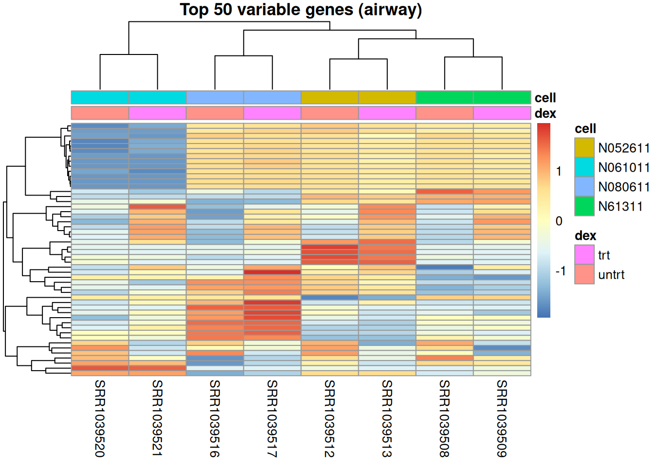
That annotation bar is the payoff in one picture: you asked for “the treatment of each sample” and got it, correctly positioned, with no bookkeeping — because the labels never left the object.
pheatmap doesn’t just color the cells — it clusters the rows and columns, reordering them so that similar genes (and similar samples) sit next to each other. It does this using only the numbers, with no knowledge of the sample labels. That is what unsupervised means: you let the data group itself, then check whether the groups line up with something you already know.
Look at how the columns group: they cluster by cell line, not by treatment — and the cell annotation bar makes it obvious. That’s the rule, not the exception. In RNA-seq the largest source of variation is often the donor (or a batch), not the effect you care about. Far from a failure, it’s exactly why analyses model the nuisance factor — fitting ~ cell + dex so the dexamethasone effect is estimated after accounting for which donor each sample came from. The annotation bars let you spot this kind of confounding at a glance, before you fit anything. The k-means chapter pushes the same unsupervised idea further, grouping genes by their expression patterns.
The same object you just subset and plotted is the object DESeq2, edgeR, limma, and dozens of other packages accept directly. A SummarizedExperiment is the lingua franca of Bioconductor — learn its shape once and every tool downstream speaks it. The next chapter builds one from scratch and shows how to save and share it.
30.6 Summary
A SummarizedExperiment bundles an assay matrix with aligned feature data (rowData) and sample data (colData) into one object that stays internally consistent when you subset — eliminating the silent desync bug that plagues loose matrices and tables. You can drive it with the same instincts you use for a data frame (dim, [, names), as long as you remember that $ reaches sample metadata and the numbers live in assay(). You toured the accessors, subset an experiment several different ways, and drew a heatmap whose annotations came for free from colData. Next you’ll build one of these objects yourself.
30.7 Exercises
The airway dataset is a good sandbox. Load a fresh copy so you’re not relying on any object created earlier:
data(airway, package = "airway")
air <- airway- How many genes (rows) and samples (columns) does
airhave? Which accessor tells you each sample’s treatment status? - Subset
airto just the untreated samples (dex == "untrt") and confirm that both the assay matrix and thecolDatashrank to match. - Pull the
countsassay for the first 5 genes and first 3 samples into a plain matrix. - Keep only genes with a total count above 100 across all samples. How many genes remain?
- Using the steps from the heatmap section, draw a heatmap of the top 20 variable genes in
air, annotated bycellline.
# 1. shape and the treatment column
dim(air)              # genes x samples
[1] 63677 8air$dex # treatment per sample (colData)[1] untrt trt untrt trt untrt trt untrt trt
Levels: trt untrt# 2. subsetting carries the metadata along
untrt <- air[, air$dex == "untrt"]
dim(untrt) # fewer columns; same number of rows[1] 63677 4[1] TRUE# 3. reach into one assay and slice it
assay(air, "counts")[1:5, 1:3] SRR1039508 SRR1039509 SRR1039512
ENSG00000000003 679 448 873
ENSG00000000005 0 0 0
ENSG00000000419 467 515 621
ENSG00000000457 260 211 263
ENSG00000000460 60 55 40[1] 15542# 5. top-20 heatmap, annotated by cell line
library(pheatmap)
lc <- log2(assay(air, "counts") + 1)
lc <- lc[rowSums(assay(air, "counts")) > 0, ]
top <- head(order(apply(lc, 1, sd), decreasing = TRUE), 20)
pheatmap(lc[top, ],
annotation_col = as.data.frame(colData(air)[, "cell", drop = FALSE]),
show_rownames = FALSE, scale = "row")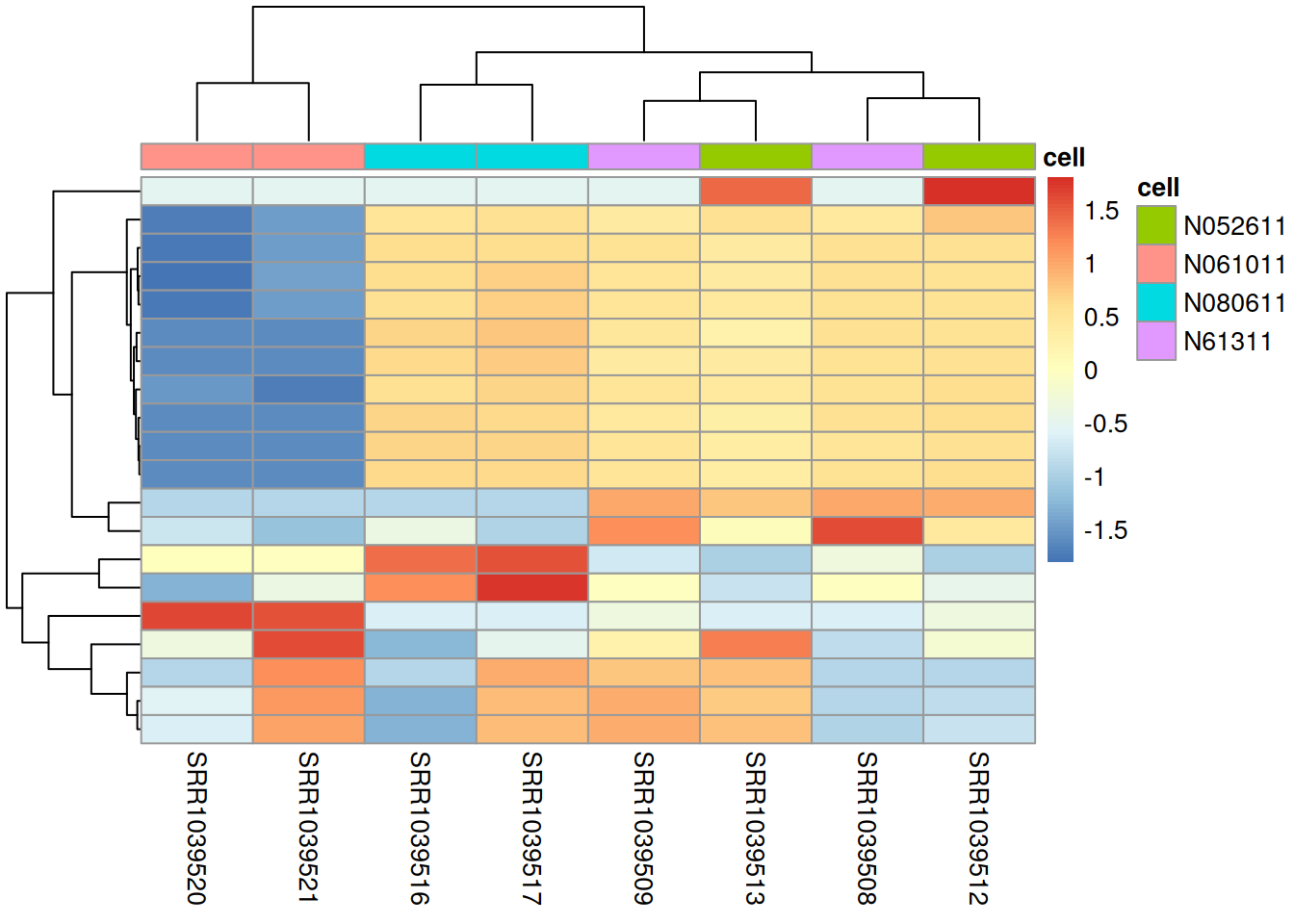
The thread through all five: you operate on the object, and the metadata stays locked to the data — exactly the guarantee a pair of loose tables can’t give you.
30.8 Reflection
- Can you state, in one sentence, the bug a
SummarizedExperimentis designed to prevent? - Given an object
se, how do you get its dimensions, a single assay, one column of sample metadata, and the treated-only samples? - Why did the heatmap’s annotation bar line up with the right samples without any extra work on your part?