32 Building and sharing a SummarizedExperiment
In the previous chapter you worked with a SummarizedExperiment someone else had assembled — the airway dataset, ready to subset and plot. But a great deal of real data does not arrive that way. It arrives as a spreadsheet: a few columns describing the genes, a wall of numeric columns holding the measurements, and the sample information living only in your head or a separate file. Turning that loose table into a proper SummarizedExperiment is one of the most useful things you can do, because from that point on the object keeps itself consistent — and it speaks the same language as every Bioconductor analysis package you’ll reach for next.
In this chapter you’ll build a SummarizedExperiment from raw parts, add a derived assay, draw a clustered heatmap, and then save and share the result so a collaborator gets everything in a single file.
32.1 What you’ll learn
By the end of this chapter you will be able to:
- Assemble a
SummarizedExperimentfrom a matrix (or several), a feature table, and a sample table — and explain the alignment rules the constructor enforces. - Add a derived assay (e.g. a normalized or log-ratio matrix) that stays aligned to the originals.
- Select informative (variable) features and draw an unsupervised clustering heatmap.
-
Save an experiment to one file and share it, provenance and all, with
saveRDS()/readRDS(). - Explain why this one object plugs into the wider Bioconductor ecosystem.
32.2 The ingredients
To construct a SummarizedExperiment you supply:
-
assays: one or more matrices (or matrix-like objects) of data — the numbers; -
rowData: aDataFramedescribing the features (rows); -
colData: aDataFramedescribing the samples (columns); - optionally
metadata: a list of anything else about the experiment.
We’ll build one from the DeRisi dataset — a classic yeast microarray time course measuring gene expression as cells exhaust their glucose and switch metabolic gears (the diauxic shift). It begins life as a plain data.frame: the first two columns identify each gene, and the rest are measurements.
library(SummarizedExperiment)
deRisi <- read.csv("https://raw.githubusercontent.com/seandavi/RBiocBook/main/data/derisi.csv")
head(deRisi)
ORF Name R1 R2 R3 R4 R5 R6 R7 R1.Bkg R2.Bkg R3.Bkg
1 YHR007C ERG11 7896 7484 14679 14617 9853 7599 6490 1155 1984 1323
2 YBR218C PYC2 12144 11177 10241 4820 4950 7047 17035 1074 1694 1243
3 YAL051W FUN43 4478 6435 6230 6848 5111 7180 4497 1140 1950 1649
4 YAL053W 6343 8243 6743 3304 3556 4694 3849 1020 1897 1196
5 YAL054C ACS1 1542 3044 2076 1695 1753 4806 10802 1082 1940 1504
6 YAL055W 1769 3243 2094 1367 1853 3580 1956 975 1821 1185
R4.Bkg R5.Bkg R6.Bkg R7.Bkg G1 G2 G3 G4 G5 G6 G7 G1.Bkg
1 1171 914 2445 981 8432 7173 11736 16798 12315 16111 13931 2404
2 876 1211 2444 742 11509 10226 13372 6500 6255 9024 6904 2148
3 1183 898 2637 927 5865 5895 5345 6302 5400 7933 5026 2422
4 881 1045 2518 697 6762 7454 6323 3595 4689 5660 4145 2107
5 1108 902 2610 980 3138 3785 2419 2114 2763 3561 1897 2405
6 851 1047 2536 698 2844 4069 2583 1651 2530 3484 1550 1674
G2.Bkg G3.Bkg G4.Bkg G5.Bkg G6.Bkg G7.Bkg
1 2561 1598 1506 1696 2667 1244
2 2527 1641 1196 1553 2569 848
3 2496 1902 1501 1644 2808 1154
4 2663 1607 1162 1577 2544 857
5 2528 1847 1445 1713 2767 1142
6 2648 1591 1114 1528 2668 870We’ll pull the three pieces out of this table one at a time.
32.2.1 rowData — feature information
The first two columns describe each gene, so they become the rowData:
rdata <- deRisi[, 1:2]
head(rdata)
ORF Name
1 YHR007C ERG11
2 YBR218C PYC2
3 YAL051W FUN43
4 YAL053W
5 YAL054C ACS1
6 YAL055W 32.2.2 colData — sample information
The sample information isn’t in the file, so we supply it ourselves. Each of the seven columns of measurements is a timepoint in the experiment:
DataFrame with 7 rows and 3 columns
       sample timepoint     hours
  <character> <integer> <numeric>
1    Sample 0         0       0.0
2    Sample 1         1       9.5
3    Sample 2         2      11.5
4    Sample 3         3      13.5
5    Sample 4         4      15.5
6    Sample 5         5      18.5
7    Sample 6         6      20.5
32.2.3 assays — the data
The DeRisi experiment recorded four different measurements for every gene at every timepoint:
| assay | description |
|---|---|
R |
Red foreground fluorescence |
G |
Green foreground fluorescence |
Rb |
Red background fluorescence |
Gb |
Green background fluorescence |
Each becomes its own matrix, sliced out of the numeric columns:
32.2.4 Aligning the names
Here is the rule that makes the whole container trustworthy. The constructor checks that the pieces line up: the row names of every assay matrix must match the row names of rowData, and the column names of every assay matrix must match the row names of colData. If they don’t, you get an error rather than a silent mismatch — the constructor refuses to build something inconsistent.
So we set those names explicitly. First the two annotation tables, keyed by gene (ORF) and by sample name:
The four assay matrices all need the same gene names on their rows and the same sample names on their columns. Rather than repeat the same two lines four times, we gather the matrices into a named list and use lapply() — which runs a function on every element of a list and returns a new list — to label them all at once:
The little function takes one matrix, sets its row and column names, and returns it; lapply() applies it to R, G, Rb, and Gb in turn. We’re left with assay_list, a named list of four correctly-labeled matrices, ready to become the object’s assays.
32.2.5 Putting it together
se <- SummarizedExperiment(assays = assay_list,
                           rowData = rdata, colData = cdata)
se
class: SummarizedExperiment
dim: 6102 7
metadata(0):
assays(4): R G Rb Gb
rownames(6102): YHR007C YBR218C ... YPR203W YPR204W
rowData names(2): ORF Name
colnames(7): Sample 0 Sample 1 ... Sample 5 Sample 6
colData names(3): sample timepoint hoursOne object now holds four aligned assays, the gene table, and the sample table. The constructor accepted it, which means everything lines up.
If you ever see an error about non-matching dimensions or names when building a SummarizedExperiment, that is the container doing its job. Check that each matrix is genes × samples (not transposed), and that its rownames/colnames match rowData/colData. The error is annoying once; the silent mismatch it prevents is annoying for the life of the paper.
32.3 Adding a derived assay
Real analysis rarely stops at the raw numbers. A natural quantity here is the background-corrected log ratio of red to green — a standard summary of two-color microarray signal. Because we compute it from assays that are already aligned, the result drops straight back into the object as a fifth assay, aligned forever:
Warning: NaNs producedassays(se)$logRatios <- logRatios
assayNames(se)[1] "R" "G" "Rb" "Gb" "logRatios"Reading the calculation from the inside out: subtract each channel’s background (R - Rb and G - Gb), divide red by green to get the ratio, and take log2 so the scale is symmetric — equal red and green gives 0, twice as much red gives +1, half as much gives −1. The assays(se)$logRatios <- ... line then tucks the new matrix into the object beside the originals.
That is a real benefit worth pausing on: you can keep raw and processed measurements in the same object, each guaranteed to refer to the same genes and samples. Reach for any of them by name:
          Sample 0     Sample 1  Sample 2   Sample 3   Sample 4 Sample 5
YHR007C -1.2204686          NaN       NaN 2.70275677  1.6545902 5.260867
YBR218C        NaN          NaN 2.9757832 2.39231742  1.9319816 3.983313
YAL051W  0.1135715          NaN       NaN        NaN -1.3681061 2.138654
YAL053W -1.3753298          NaN       NaN 0.05044902  1.0906497 5.215440
YAL054C  0.2706476  0.333657387 0.0000000 0.31420165  0.3165815      NaN
YAL055W  0.6209723 -0.001745548 0.2683547 0.11082813  0.4931189      NaN
         Sample 6
YHR007C 4.8223618
YBR218C       NaN
YAL051W 1.2205754
YAL053W 0.8875253
YAL054C       NaN
YAL055W       NaN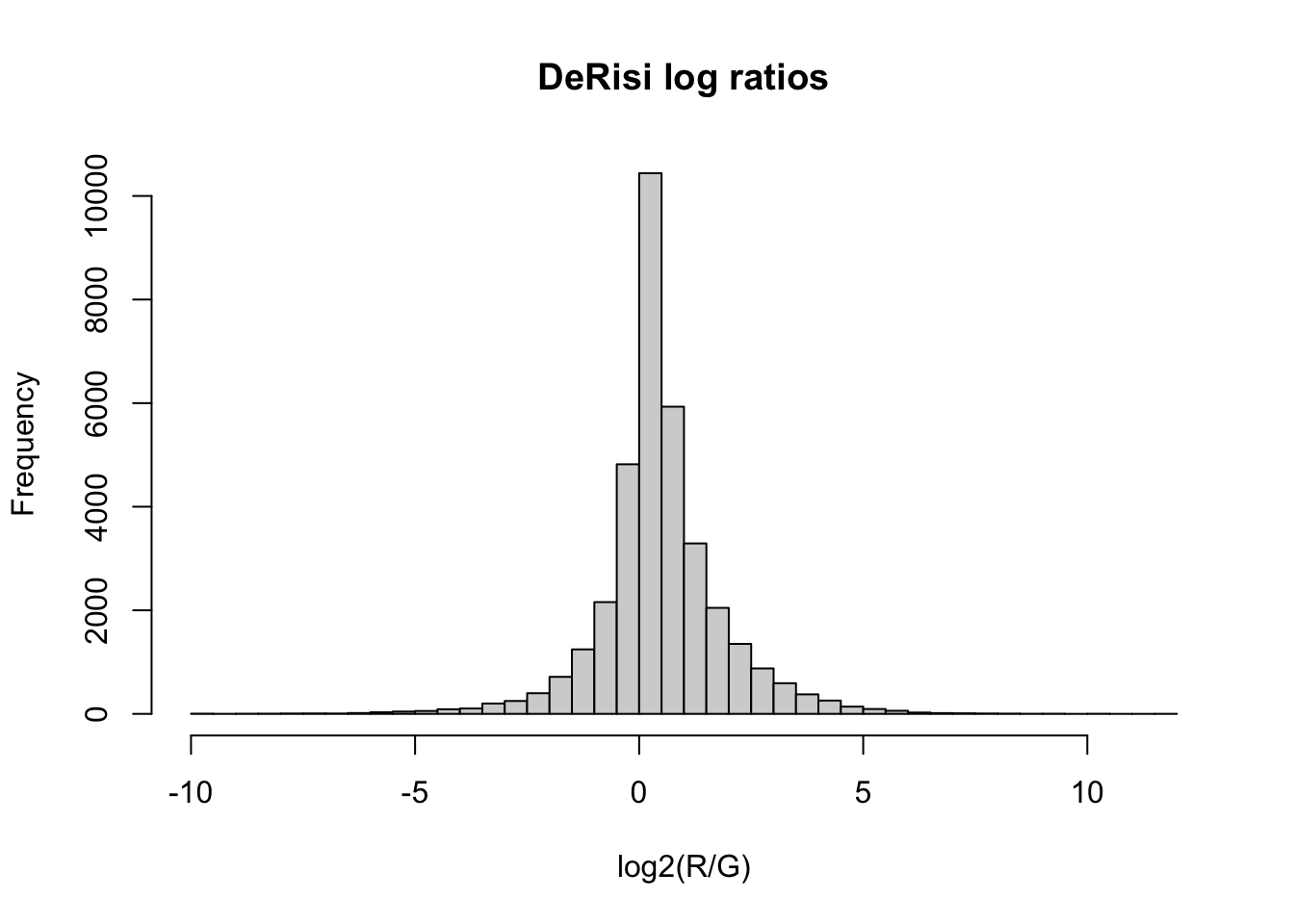
32.4 A clustering heatmap of informative genes
With 6,400 genes, no heatmap can show them all — nor would you want it to. As in the previous chapter, we keep the variable genes, because a gene whose log ratio barely moves across the time course carries no information about the diauxic shift; the genes that rise and fall are the informative ones. We rank by standard deviation and keep the top 50.
The log-ratio calculation produces some non-finite values (a background-corrected signal can go negative, and log2 of a negative number is NaN), so we first keep only genes measured cleanly at every timepoint:
[1] 50 7That filter line reads inside-out: is.finite(lr) is a TRUE/FALSE matrix marking the good values; !is.finite(lr) flips it to mark the bad ones; rowSums(...) counts the bad values in each gene’s row; and == 0 keeps only the genes with none — a clean log ratio at all seven timepoints. Then apply(lr, 1, sd) gives each surviving gene’s standard deviation across the timepoints, and head(order(..., decreasing = TRUE), 50) keeps the 50 most variable.
Now the heatmap. Two deliberate choices: we don’t cluster the columns (cluster_cols = FALSE) so the samples stay in time order and we can read each gene’s trajectory left to right; and we do cluster the rows, which groups genes that move together. The column annotation — the time in hours — comes straight from colData.
library(pheatmap)
ann <- as.data.frame(colData(se)[, "hours", drop = FALSE])
pheatmap(lr_top,
         cluster_cols = FALSE,          # keep samples in time order
         cluster_rows = TRUE,           # group co-regulated genes
         annotation_col = ann,
         show_rownames = FALSE,
         scale = "row",
         main = "Top 50 variable genes (DeRisi)")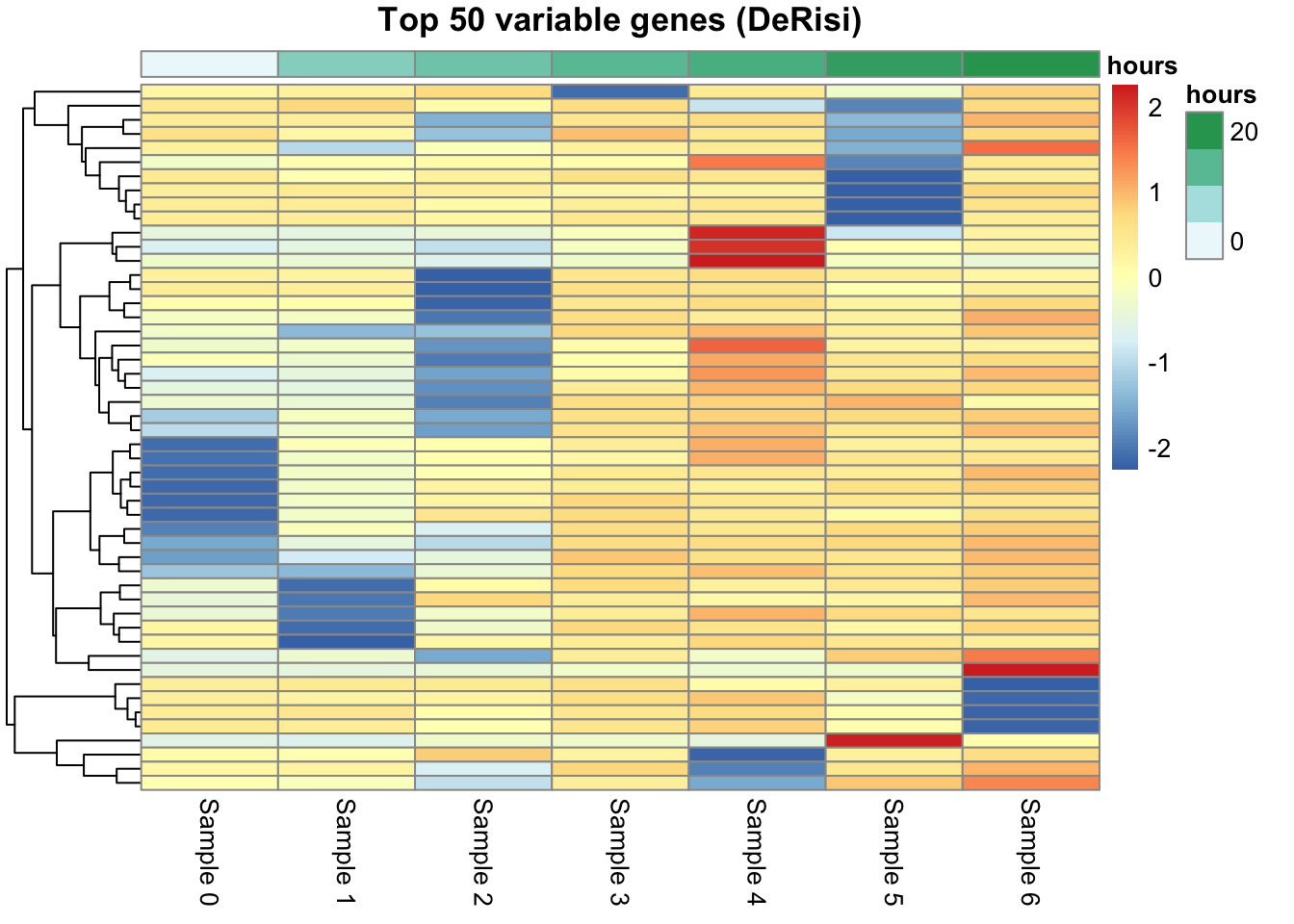
Clustering the rows here groups genes purely by how similarly their expression moves over time, with no labels supplied — the same unsupervised idea you met in the previous chapter, now pointed at features instead of samples. Blocks of genes that rise together (or fall together) across the diauxic shift show up as bands. That is exactly the structure the k-means chapter sets out to find formally on this very dataset; the heatmap is the quick, visual version of the same question.
32.5 Saving and sharing
Here is the part that makes a collaborator’s day. Your experiment — four raw assays, a derived one, the gene table, the sample table, and any notes — is a single R object. Save it to a single file:
Anyone who receives that file reads it back and has everything, already aligned, with nothing to re-link:
se2 <- readRDS(path)
se2
class: SummarizedExperiment
dim: 6102 7
metadata(0):
assays(5): R G Rb Gb logRatios
rownames(6102): YHR007C YBR218C ... YPR203W YPR204W
rowData names(2): ORF Name
colnames(7): Sample 0 Sample 1 ... Sample 5 Sample 6
colData names(3): sample timepoint hoursNo “which spreadsheet had the sample labels?”, no “are the columns in the same order?”. The object is self-describing. Stash provenance in metadata() and it rides along too:
$processing
[1] "background-corrected log2 ratios; built in the RBioc Book"

$date
[1] "2026-06-06"
This is also how published datasets are distributed: many arrive as ready-made SummarizedExperiment objects through Bioconductor’s ExperimentHub and data packages (the airway package from the last chapter is exactly this). You load one line and get an analysis-ready object — because the author saved it in this shape.
32.6 Why this is worth it: the ecosystem payoff
Step back and ask what you actually gained by building this object instead of keeping a few matrices around.
- It can’t silently desync. Every subset, every new assay, stays aligned.
- It carries its own context. Feature annotation, sample annotation, and experiment notes travel with the numbers, in one file.
-
It is the common currency of Bioconductor. This is the big one. Hundreds of analysis packages —
DESeq2andedgeRandlimmafor differential expression,scranandscaterfor single cell, and many more — take aSummarizedExperimentand hand one back. You don’t reshape your data for each tool; you build the object once and plug it into all of them. -
It is the root of a family. The
SingleCellExperimentyou’ll meet in the single-cell chapter and theTreeSummarizedExperimentin the microbiome chapter are bothSummarizedExperiments with extra parts bolted on. Learn this shape once and those feel familiar immediately. The GEOquery chapter and the k-means chapter both hand you data in exactly this form.
Build it once; everything downstream speaks the same language.
32.7 Summary
You took a flat spreadsheet and assembled it into a SummarizedExperiment — extracting rowData, supplying colData, building four assay matrices, and letting the constructor enforce that they all line up. You added a derived log-ratio assay that stays aligned, drew an unsupervised clustering heatmap of the most informative genes, and saved the whole thing to one self-describing file that carries its provenance. Most importantly, you now hold an object that the rest of the Bioconductor ecosystem accepts directly.
32.8 Exercises
-
Build a tiny one. Create a
SummarizedExperimentfrom a 4 × 3 matrix of your choosing, arowDatawith agenecolumn, and acolDatawith agroupcolumn. Confirm itsdim(). -
Break it on purpose. Try to build a
SummarizedExperimentwhere the assay has 3 columns butcolDatahas 4 rows. What happens, and why is that a good thing? -
Add a derived assay. To the DeRisi
se, add an assay calledRcorrequal toR - Rb(red minus red background). Confirm it appears inassayNames(se). -
Save and reload. Save the DeRisi
seto a temporary file, read it back, and confirm the assay names andmetadata()survived.
# 1. a minimal SummarizedExperiment
m <- matrix(1:12, nrow = 4,
            dimnames = list(paste0("g", 1:4), paste0("s", 1:3)))
rd <- DataFrame(gene = paste0("g", 1:4), row.names = paste0("g", 1:4))
cd <- DataFrame(group = c("a", "a", "b"), row.names = paste0("s", 1:3))
tiny <- SummarizedExperiment(assays = list(counts = m), rowData = rd, colData = cd)
dim(tiny)
[1] 4 3# 2. mismatched dimensions -> the constructor errors (a feature, not a bug):
# it refuses to build an object whose pieces don't line up, so you can never
# end up with sample labels pointing at the wrong columns.
try(SummarizedExperiment(assays = list(x = m[, 1:3]),
colData = DataFrame(group = letters[1:4])))Error in `rownames<-`(`*tmp*`, value = .get_colnames_from_first_assay(assays)) :
invalid rownames length# 3. a derived assay, aligned automatically
assays(se)$Rcorr <- assay(se, "R") - assay(se, "Rb")
assayNames(se)[1] "R" "G" "Rb" "Gb" "logRatios" "Rcorr" # 4. round-trip through a file
f <- tempfile(fileext = ".rds")
saveRDS(se, f)
back <- readRDS(f)
assayNames(back)[1] "R" "G" "Rb" "Gb" "logRatios" "Rcorr" metadata(back)$processing
[1] "background-corrected log2 ratios; built in the RBioc Book"
$date
[1] "2026-06-06"