library(rtracklayer)
library(GenomicRanges)
library(ggplot2)
library(dplyr)

theme_set(theme_minimal())28 Genomic ranges with real ChIP-seq peaks
CTCF is one of the most important architectural proteins in the human genome. It binds thousands of sites across the chromosomes, where it helps fold DNA into loops and marks the boundaries between active and silent regions. So a natural question for a biologist is: where does CTCF actually bind?
A ChIP-seq experiment answers that question by handing you a list of genomic intervals — the peaks where the protein was detected. In this chapter you’ll take a real CTCF peak set from the ENCODE project, load it into R, and learn the tools you need to explore it: how genomic coordinates are stored on disk, how to import them, and how to ask questions like “how wide are these peaks?” and “where exactly is the center of each one?”
This chapter focuses on the real-data workflow — file formats, importing, and exploring. For the full catalog of range operations (set operations, overlaps, nearest-feature searches, gene models), see the Genomic ranges and features chapter, which builds GRanges objects by hand and works through those methods systematically. Here we keep our hands on a real dataset.
28.1 What you’ll learn
- Read the BED / narrowPeak file format and explain its coordinate system.
- Import a peak file from a URL into a
GRangesobject withrtracklayer. - Use the accessor functions (
seqnames(),start(),width(),mcols()) to pull information out of aGRanges. - Interpret the distribution of peak widths and what it tells you about the peak caller.
- Manipulate ranges with
shift(),resize(), andflank()to build the windows downstream analyses need. - Compute and visualize read coverage along a chromosome.
28.2 The BED file format
Genomic intervals are most often stored in BED (Browser Extensible Data) format: a tab-delimited text file where each line is one feature. The first three columns are required and define the interval itself:
-
chrom — chromosome name (e.g.
chr1,chrX). - chromStart — start position.
- chromEnd — end position.
Optional columns can follow: a feature name, a score, the strand, and several more. Peak callers extend BED with extra columns (signal values, p-values); that flavor is called narrowPeak, and it’s what our ENCODE file uses.
WarningBED is 0-based; R is 1-based
This is the single most common source of off-by-one bugs in genomics, so it is worth burning into memory. BED files use a 0-based, half-open coordinate system: counting starts at 0, the start is included, and the end is excluded. R — and the GRanges objects you’ll build from these files — use a 1-based, fully-closed system: counting starts at 1 and both ends are included.
Take the BED line chr1 1000 2000. In BED that means the 1000 bases spanning the interval [1000, 2000). When rtracklayer imports it, the start becomes 1001 (shifted up by one) and the end stays 2000, giving the same 1000 bases but now written as 1001-2000 in 1-based coordinates. The width is identical (2000 - 1000 = 1000); only the numbering differs. The good news: rtracklayer does this conversion for you. The trap is doing the arithmetic yourself on the raw file and being off by one.
28.3 Loading the libraries
28.4 Importing the CTCF peaks
We’ll use a CTCF ChIP-seq peak file from ENCODE. It lives at a URL, and rtracklayer::import() can read straight from that URL — no need to download it by hand first.
Before we use the convenient importer, let’s peek at the raw file so you can see that it really is just a table of numbers and text:
bed_url <- "https://www.encodeproject.org/files/ENCFF960ZGP/@@download/ENCFF960ZGP.bed.gz"

# Read the raw file as a plain table just to see its shape
ctcf_peaks_raw <- readr::read_table(bed_url, col_names = FALSE)
── Column specification ────────────────────────────────────────────────────────
cols(
  X1 = col_character(),
  X2 = col_double(),
  X3 = col_double(),
  X4 = col_character(),
  X5 = col_double(),
  X6 = col_character(),
  X7 = col_double(),
  X8 = col_double(),
  X9 = col_double(),
  X10 = col_double()
)head(ctcf_peaks_raw)# A tibble: 6 × 10
X1 X2 X3 X4 X5 X6 X7 X8 X9 X10
<chr> <dbl> <dbl> <chr> <dbl> <chr> <dbl> <dbl> <dbl> <dbl>
1 chr2 238305323 238305539 . 1000 . 7.70 -1 0.274 108
2 chr20 49982706 49982922 . 541 . 8.72 -1 0.466 108
3 chr15 39921015 39921231 . 672 . 9.08 -1 0.547 108
4 chr8 6708273 6708489 . 560 . 9.86 -1 0.662 108
5 chr9 136645956 136646172 . 584 . 10.2 -1 0.751 108
6 chr7 47669294 47669510 . 614 . 10.5 -1 0.807 108Each row is one peak, and you can see the chromosome, start, and end in the first three columns followed by the narrowPeak extras. Now let’s import it properly into a GRanges object, which is the data structure built for genomic intervals:
ctcf_peaks <- rtracklayer::import(bed_url, format = "narrowPeak")
ctcf_peaks
GRanges object with 43865 ranges and 6 metadata columns:
seqnames ranges strand | name score
<Rle> <IRanges> <Rle> | <character> <numeric>
[1] chr2 238305324-238305539 * | <NA> 1000
[2] chr20 49982707-49982922 * | <NA> 541
[3] chr15 39921016-39921231 * | <NA> 672
[4] chr8 6708274-6708489 * | <NA> 560
[5] chr9 136645957-136646172 * | <NA> 584
... ... ... ... . ... ...
[43861] chr11 66222736-66222972 * | <NA> 1000
[43862] chr10 75235956-75236225 * | <NA> 1000
[43863] chr16 57649100-57649347 * | <NA> 1000
[43864] chr17 37373596-37373838 * | <NA> 1000
[43865] chr12 53676108-53676355 * | <NA> 1000
signalValue pValue qValue peak
<numeric> <numeric> <numeric> <integer>
[1] 7.70385 -1 0.27378 108
[2] 8.71626 -1 0.46571 108
[3] 9.07638 -1 0.54697 108
[4] 9.86234 -1 0.66189 108
[5] 10.15488 -1 0.75082 108
... ... ... ... ...
[43861] 478.640 -1 4.87574 124
[43862] 480.183 -1 4.87574 141
[43863] 491.081 -1 4.87574 116
[43864] 491.991 -1 4.87574 127
[43865] 494.303 -1 4.87574 126
-------
seqinfo: 26 sequences from an unspecified genome; no seqlengths
NoteWhat
format = "narrowPeak" gives you
Telling import() that the file is narrowPeak does two helpful things. First, it applies the 0-based-to-1-based conversion described above, so the start, end, and width you see are already in R’s coordinate system. Second, it parses the peak-caller columns into named metadata: signalValue, pValue, qValue, and peak (the offset of the summit within the peak). Those land in the metadata columns of the GRanges, where you can reach them with $.
28.5 Looking inside a GRanges
A GRanges keeps the ranges (chromosome, start, end, strand) separate from the metadata (everything else). You pull each part out with an accessor function.
length(ctcf_peaks) # how many peaks?[1] 43865factor-Rle of length 6 with 6 runs
Lengths: 1 1 1 1 1 1
Values : chr2 chr20 chr15 chr8 chr9 chr7
Levels(26): chr2 chr20 chr15 ... chr1_KI270714v1_random chrUn_GL000219v1[1] 238305324 49982707 39921016 6708274 136645957 47669295[1] 238305539 49982922 39921231 6708489 136646172 47669510[1] 216 216 216 216 216 216So this file contains 43865 CTCF peaks. The widths vary, but let’s look at the whole distribution rather than the first six values:
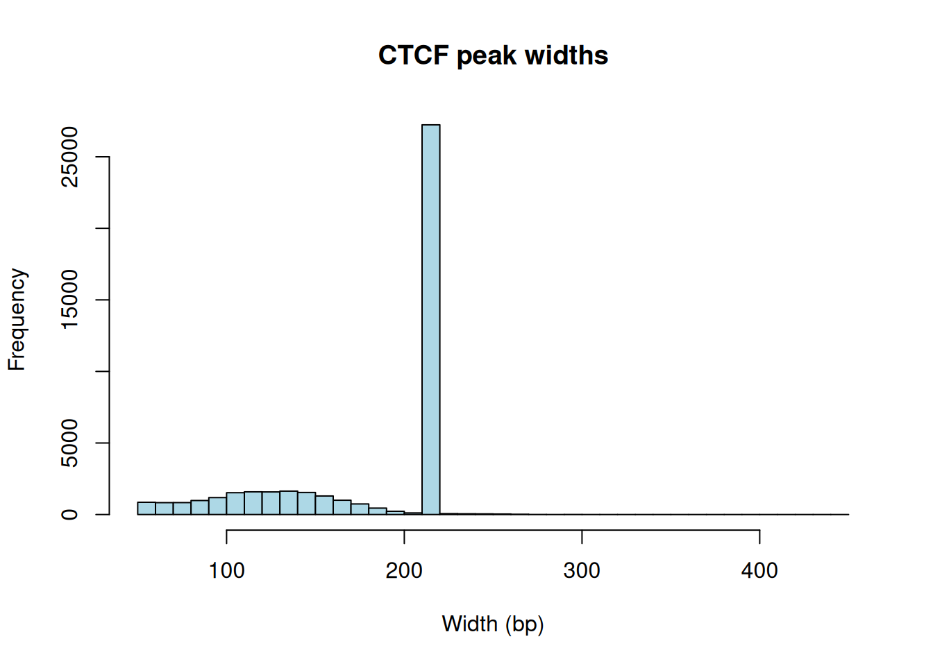
Figure 28.1 has a striking feature: a tall spike at one particular width rather than a smooth spread. That’s not biology — it’s the peak caller. Many ChIP-seq pipelines report peaks at a fixed width (here around 200 bp) centered on the detected summit, so the same number shows up over and over. When you see a histogram like this, read it as a signature of how the data were processed, not as a property of CTCF itself.
The metadata sits in a separate table you reach with mcols():
DataFrame with 6 rows and 6 columns
         name     score signalValue    pValue    qValue      peak
  <character> <numeric>   <numeric> <numeric> <numeric> <integer>
1          NA      1000     7.70385        -1   0.27378       108
2          NA       541     8.71626        -1   0.46571       108
3          NA       672     9.07638        -1   0.54697       108
4          NA       560     9.86234        -1   0.66189       108
5          NA       584    10.15488        -1   0.75082       108
6          NA       614    10.46015        -1   0.80676       108
These are the narrowPeak columns. You can pull one out directly with $ — for example the signalValue, which measures how strong the binding signal was at each peak:
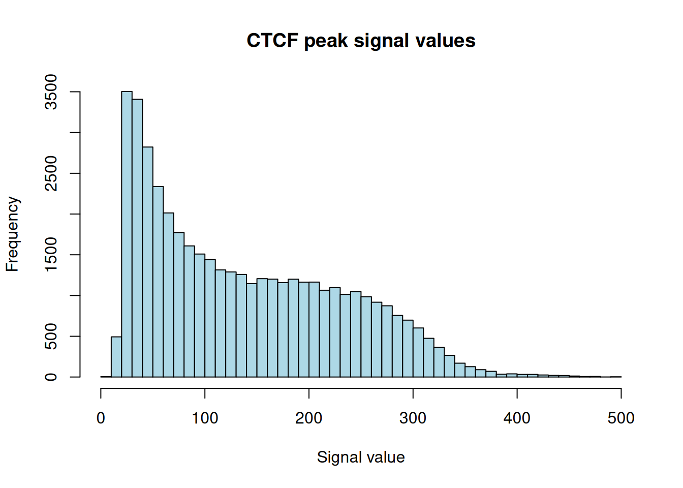
Figure 28.2 is right-skewed: most peaks carry a modest signal, with a long tail of much stronger binding sites. That shape is typical of ChIP-seq — a handful of high-confidence sites and many weaker ones — and it’s why people often filter on signalValue before downstream work.
28.6 Some quick summaries
How many peaks, on how many chromosomes, and how wide? A few small expressions answer this more clearly than a wall of printed text:
The median width sits right at the spike we saw in Figure 28.1, confirming that most peaks share the caller’s fixed width. We can also count peaks per chromosome:
peaks_per_chr <- table(seqnames(ctcf_peaks))
head(as.data.frame(peaks_per_chr), 10)
Var1 Freq
1 chr2 3332
2 chr20 1236
3 chr15 1431
4 chr8 1935
5 chr9 1820
6 chr7 2140
7 chr4 2030
8 chr12 2274
9 chr5 2355
10 chr22 873Larger chromosomes generally carry more peaks, which makes sense: more DNA means more potential binding sites.
28.7 Where is each peak?
Three quantities you’ll reach for constantly are the start, the end, and the center of each peak. The center is especially useful — motif analyses and fixed-width windows are usually built around it.
[1] 238305432 49982815 39921124 6708382 136646065peak_centers now holds the midpoint of every peak, ready to anchor a window.
28.8 Reshaping ranges
Three functions cover most of the range-reshaping you’ll do on a peak set: shift() slides a range, resize() changes its width, and flank() builds a neighbouring region. They all return a new GRanges and leave the original untouched.
28.8.1 Shifting
shift() moves every range by a fixed number of bases without changing its width:
peaks_shifted <- shift(ctcf_peaks, 100)   # slide right by 100 bp

ctcf_peaks[1]
GRanges object with 1 range and 6 metadata columns:
seqnames ranges strand | name score signalValue
<Rle> <IRanges> <Rle> | <character> <numeric> <numeric>
[1] chr2 238305324-238305539 * | <NA> 1000 7.70385
pValue qValue peak
<numeric> <numeric> <integer>
[1] -1 0.27378 108
-------
seqinfo: 26 sequences from an unspecified genome; no seqlengthspeaks_shifted[1]GRanges object with 1 range and 6 metadata columns:
seqnames ranges strand | name score signalValue
<Rle> <IRanges> <Rle> | <character> <numeric> <numeric>
[1] chr2 238305424-238305639 * | <NA> 1000 7.70385
pValue qValue peak
<numeric> <numeric> <integer>
[1] -1 0.27378 108
-------
seqinfo: 26 sequences from an unspecified genome; no seqlengthsThe start and end of the first peak both moved up by 100, and the width is unchanged — exactly what “shift” should do.
28.8.2 Resizing
resize() sets every range to a chosen width. The fix argument says which point to hold still while the width changes. Resizing all peaks to a common width is the standard way to build comparable windows:
peaks_200bp <- resize(ctcf_peaks, width = 200, fix = "center")

peaks_200bp[1]
GRanges object with 1 range and 6 metadata columns:
seqnames ranges strand | name score signalValue
<Rle> <IRanges> <Rle> | <character> <numeric> <numeric>
[1] chr2 238305332-238305531 * | <NA> 1000 7.70385
pValue qValue peak
<numeric> <numeric> <integer>
[1] -1 0.27378 108
-------
seqinfo: 26 sequences from an unspecified genome; no seqlengths[1] TRUEFixing on "center" keeps each peak’s midpoint in place and grows or shrinks it symmetrically — so a downstream tool sees uniform 200 bp windows centered on the binding sites.
28.8.3 Flanking
flank() returns the region beside a range — useful for grabbing the DNA just upstream or downstream of a peak:
upstream_1kb <- flank(ctcf_peaks, width = 1000, start = TRUE)

ctcf_peaks[1]
GRanges object with 1 range and 6 metadata columns:
seqnames ranges strand | name score signalValue
<Rle> <IRanges> <Rle> | <character> <numeric> <numeric>
[1] chr2 238305324-238305539 * | <NA> 1000 7.70385
pValue qValue peak
<numeric> <numeric> <integer>
[1] -1 0.27378 108
-------
seqinfo: 26 sequences from an unspecified genome; no seqlengthsupstream_1kb[1]GRanges object with 1 range and 6 metadata columns:
seqnames ranges strand | name score signalValue
<Rle> <IRanges> <Rle> | <character> <numeric> <numeric>
[1] chr2 238304324-238305323 * | <NA> 1000 7.70385
pValue qValue peak
<numeric> <numeric> <integer>
[1] -1 0.27378 108
-------
seqinfo: 26 sequences from an unspecified genome; no seqlengthsThe flanking range is the 1000 bp sitting immediately before the start of the first peak — the kind of window you might scan for a neighbouring promoter.
NoteOverlaps and grouped operations live next door
Once you have peaks and other features (genes, promoters, other peak sets), the next question is usually which ones overlap? The findOverlaps() and nearest() functions, set operations like intersect(), and grouped operations over a GRangesList are covered in depth in the Genomic ranges and features chapter. We don’t repeat them here so we can stay focused on the real-data import workflow.
28.9 Coverage
Coverage counts how many ranges overlap each position along a chromosome. It’s the foundation of peak calling: pile up sequencing reads, and the tall stacks are where the protein bound. Let’s build a toy example by scattering random reads across a one-megabase stretch and counting the pile-up.
set.seed(42)   # reproducible random reads
chrom_length <- 1000000
num_reads    <- 100000
read_length  <- 50

random_starts <- sample(seq_len(chrom_length - read_length + 1),
                         num_reads, replace = TRUE)
random_reads  <- GRanges(seqnames = "chr1",
                         ranges = IRanges(start = random_starts,
                                          end = random_starts + read_length - 1))
random_reads
GRanges object with 100000 ranges and 0 metadata columns:
seqnames ranges strand
<Rle> <IRanges> <Rle>
[1] chr1 61413-61462 *
[2] chr1 54425-54474 *
[3] chr1 623844-623893 *
[4] chr1 74362-74411 *
[5] chr1 46208-46257 *
... ... ... ...
[99996] chr1 663489-663538 *
[99997] chr1 886082-886131 *
[99998] chr1 933222-933271 *
[99999] chr1 486340-486389 *
[100000] chr1 177556-177605 *
-------
seqinfo: 1 sequence from an unspecified genome; no seqlengthsThe coverage() function turns those reads into a per-base count. It returns an Rle (run-length encoded) object — a compact way to store long stretches of repeated values:
RleList of length 1
$chr1
integer-Rle of length 1000000 with 173047 runs
  Lengths:  7  1  6  3  8  8  1  1 22  1  4 ...  3  1  2  8 12 23  5  2  8  6
  Values :  0  1  3  4  5  6  7  8  9  8  6 ...  3  2  3  4  5  4  3  2  1  0
Let’s look at the coverage across the first 10,000 bases:
plot(random_coverage[[1]][1:10000], type = "h", col = "blue",
     main = "Coverage of random reads", xlab = "Position", ylab = "Coverage")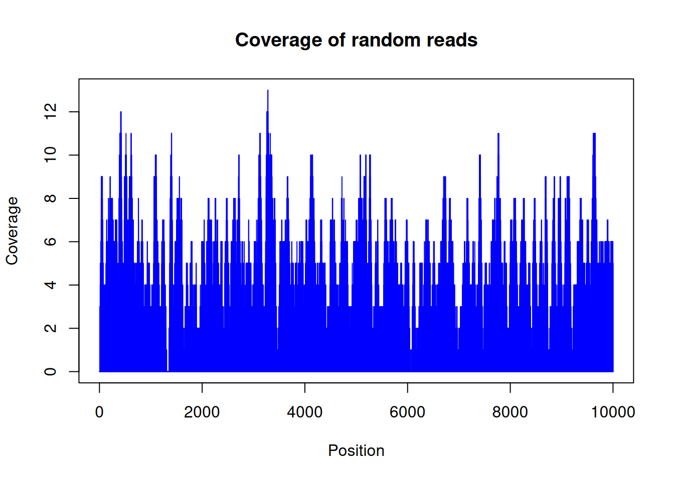
Figure 28.3 looks like noise, and that’s the point: because we placed the reads at random, the coverage hovers around a constant average with no real peaks. Real ChIP-seq data would show tall, localized spikes where the protein bound — those spikes are what a peak caller hunts for, and their absence here is exactly what “no signal” should look like.
We can also ask how the coverage is distributed across all positions:
hist(as.numeric(random_coverage[[1]]),
     main = "Coverage distribution", xlab = "Coverage", ylab = "Frequency",
     col = "lightblue")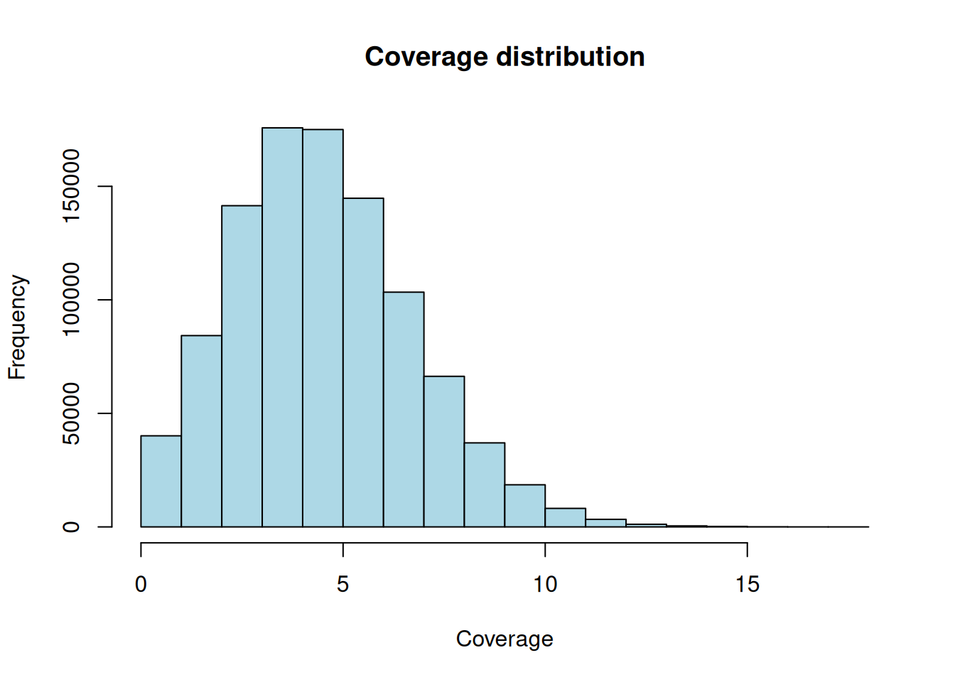
Figure 28.4 is a tidy bell-ish hump centered on the average depth. With 1e+05 reads of length 50 spread over 1e+06 bases, the expected coverage is about 5x — right where the hump sits. Random reads give random, evenly-spread coverage; biological signal is what makes that distribution lumpy.
28.10 Exercises
Use the ctcf_peaks object you imported above. Each solution names the accessor or function that does the job.
-
Wide peaks. How many CTCF peaks are wider than 250 bp?
-
Fixed-width windows. Build a new
GRangesof 500 bp windows centered on each peak, and confirm every window is exactly 500 bp wide. -
Peak centers. Compute the center position of every peak and report the median center.
-
Fraction on chr1. What fraction of all CTCF peaks fall on
chr1?NoteSolutionComparing
seqnames()to"chr1"gives a TRUE/FALSE vector;mean()of a logical vector is the proportion that are TRUE — a handy idiom for “what fraction satisfy this condition?”
28.11 Summary
You can now take a real peak set from file to insight:
- Read a BED/narrowPeak file and explain its 0-based, half-open coordinate system — and why R’s 1-based coordinates differ.
-
Import peaks into a
GRangesstraight from a URL withrtracklayer::import(..., format = "narrowPeak"), which handles the coordinate conversion and parses the metadata columns. -
Explore the object with
seqnames(),start(),end(),width(), andmcols(), and read its width and signal distributions as fingerprints of the peak caller and the biology. -
Reshape ranges with
shift(),resize(), andflank()to build the windows downstream tools expect. - Compute coverage and recognize that random reads give flat coverage, while biological signal makes it lumpy.
For overlaps, nearest-feature searches, set operations, and gene models, continue to the Genomic ranges and features chapter, which treats those operations in full.