2 * 3 [1] 64 - 1 [1] 3# this obeys order-of-operations
6 / (4 - 1) [1] 2In this chapter, we’re going to get an introduction to the R language, so we can dive right into programming. We’re going to create a pair of virtual dice that can generate random numbers. No need to worry if you’re new to programming. We’ll return to many of the concepts here in more detail later.
To simulate a pair of dice, we need to break down each die into its essential features. A die can only show one of six numbers: 1, 2, 3, 4, 5, and 6. We can capture the die’s essential characteristics by saving these numbers as a group of values in the computer. Let’s save these numbers first and then figure out a way to “roll” our virtual die.
The RStudio interface is simple. You type R code into the bottom line of the RStudio console pane and then click Enter to run it. The code you type is called a command, because it will command your computer to do something for you. The line you type it into is called the command line.
When you type a command at the prompt and hit Enter, your computer executes the command and shows you the results. Then RStudio displays a fresh prompt for your next command. For example, if you type 1 + 1 and hit Enter, RStudio will display:
> 1 + 1
[1] 2
>
You’ll notice that a [1] appears next to your result. R is just letting you know that this line begins with the first value in your result. Some commands return more than one value, and their results may fill up multiple lines. For example, the command 100:130 returns 31 values; it creates a sequence of integers from 100 to 130. Notice that new bracketed numbers appear at the start of the second and third lines of output. These numbers just mean that the second line begins with the 14th value in the result, and the third line begins with the 25th value. You can mostly ignore the numbers that appear in brackets:
> 100:130
 [1] 100 101 102 103 104 105 106 107 108 109 110 111 112
[14] 113 114 115 116 117 118 119 120 121 122 123 124 125
[25] 126 127 128 129 130The colon operator (:) returns every integer between two integers. It is an easy way to create a sequence of numbers.
In some languages, like C, Java, and FORTRAN, you have to compile your human-readable code into machine-readable code (often 1s and 0s) before you can run it. If you’ve programmed in such a language before, you may wonder whether you have to compile your R code before you can use it. The answer is no. R is a dynamic programming language, which means R automatically interprets your code as you run it.
If you type an incomplete command and press Enter, R will display a + prompt, which means R is waiting for you to type the rest of your command. Either finish the command or hit Escape to start over:
> 5 -
+
+ 1
[1] 4
If you type a command that R doesn’t recognize, R will return an error message. If you ever see an error message, don’t panic. R is just telling you that your computer couldn’t understand or do what you asked it to do. You can then try a different command at the next prompt:
> 3 % 5
Error: unexpected input in "3 % 5"
>Whenever you get an error message in R, consider googling the error message. You’ll often find that someone else has had the same problem and has posted a solution online. Simply cutting-and-pasting the error message into a search engine will often work
Once you get the hang of the command line, you can easily do anything in R that you would do with a calculator. For example, you could do some basic arithmetic:
2 * 3 [1] 64 - 1 [1] 3# this obeys order-of-operations
6 / (4 - 1) [1] 2R treats the hashtag character, #, in a special way; R will not run anything that follows a hashtag on a line. This makes hashtags very useful for adding comments and annotations to your code. Humans will be able to read the comments, but your computer will pass over them. The hashtag is known as the commenting symbol in R.
Some R commands may take a long time to run. You can cancel a command once it has begun by pressing ctrl + c or by clicking the “stop sign” if it is available in Rstudio. Note that it may also take R a long time to cancel the command.
That’s the basic interface for executing R code in RStudio. Think you have it? If so, try doing these simple tasks. If you execute everything correctly, you should end up with the same number that you started with:
10 + 2[1] 1212 * 3[1] 3636 - 6[1] 3030 / 3[1] 10Now that you know how to use R, let’s use it to make a virtual die. The : operator from a couple of pages ago gives you a nice way to create a group of numbers from one to six. The : operator returns its results as a vector (we are going to work with vectors in more detail), a one-dimensional set of numbers:
1:6
## 1 2 3 4 5 6
That’s all there is to how a virtual die looks! But you are not done yet. Running 1:6 generated a vector of numbers for you to see, but it didn’t save that vector anywhere for later use. If we want to use those numbers again, we’ll have to ask your computer to save them somewhere. You can do that by creating an R object.
R lets you save data by storing it inside an R object. What is an object? Just a name that you can use to call up stored data. For example, you can save data into an object like a or b. Wherever R encounters the object, it will replace it with the data saved inside, like so:
a <- 1
a
[1] 1a + 2[1] 3<, followed by a minus sign, -, to save data into it. This combination looks like an arrow, <-. R will make an object, give it your name, and store in it whatever follows the arrow. So a <- 1 stores 1 in an object named a.a, R tells you on the next line.a previously stored the value of 1, you’re now adding 1 to 2.Everything that you type into the R console can be assigned to one of two categories:
An expression is a command that tells R to do something. For example, 1 + 2 is an expression that tells R to add 1 and 2. When you type an expression into the R console, R will evaluate the expression and return the result. For example, if you type 1 + 2 into the R console, R will return 3. Expressions can have “side effects” but they don’t explicitly result in anything being added to R memory.
While using R as a calculator is interesting, to do useful and interesting things, we need to assign values to objects. To create objects, we need to give it a name followed by the assignment operator <- (or, entirely equivalently, =) and the value we want to give it:
weight_kg <- 55So, for another example, the following code would create an object named die that contains the numbers one through six. To see what is stored in an object, just type the object’s name by itself:
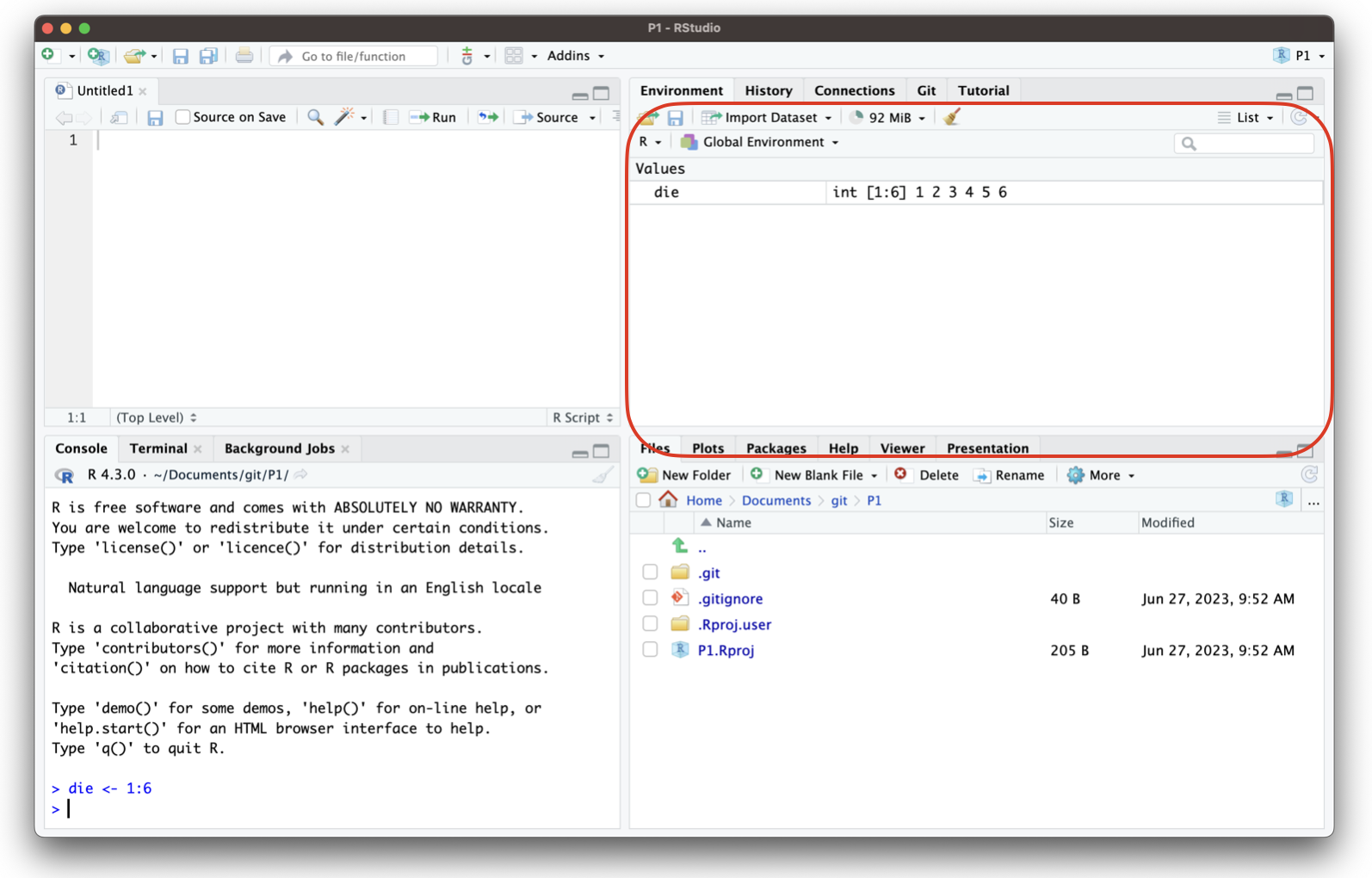
die <- 1:6
die
[1] 1 2 3 4 5 6When you create an object, the object will appear in the environment pane of RStudio, as shown in Figure 4.2. This pane will show you all of the objects you’ve created since opening RStudio.
You can name an object in R almost anything you want, but there are a few rules. First, a name cannot start with a number. Second, a name cannot use some special symbols, like ^, !, $, @, +, -, /, or *:
| Good names | Names that cause errors |
|---|---|
| a | 1trial |
| b | $ |
| FOO | ^mean |
| my_var | 2nd |
| .day | !bad |
R is case-sensitive, so name and Name will refer to different objects:
> Name = 0
> Name + 1
[1] 1
> name + 1
Error: object 'name' not found
The error above is a common one!
Finally, R will overwrite any previous information stored in an object without asking you for permission. So, it is a good idea to not use names that are already taken:
my_number <- 1
my_number
[1] 1my_number <- 999
my_number[1] 999You can see which object names you have already used with the function ls:
ls()Your environment will contain different names than mine, because you have probably created different objects.
You can also see which names you have used by examining RStudio’s environment pane.
We now have a virtual die that is stored in the computer’s memory and which has a name that we can use to refer to it. You can access it whenever you like by typing the word die.
So what can you do with this die? Quite a lot. R will replace an object with its contents whenever the object’s name appears in a command. So, for example, you can do all sorts of math with the die. Math isn’t so helpful for rolling dice, but manipulating sets of numbers will be your stock and trade as a data scientist. So let’s take a look at how to do that:
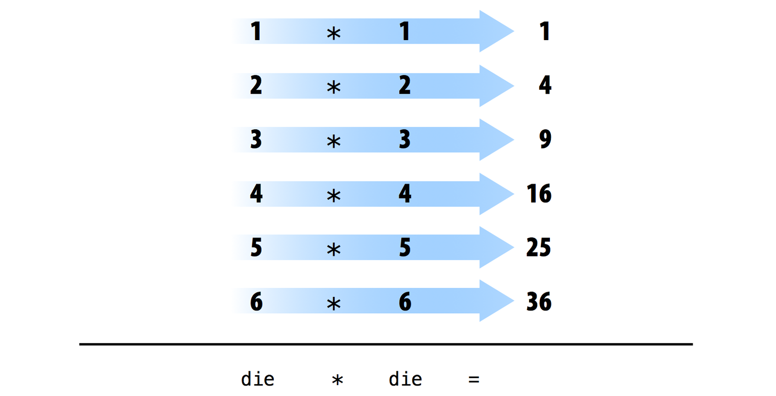
die - 1[1] 0 1 2 3 4 5die / 2[1] 0.5 1.0 1.5 2.0 2.5 3.0die * die[1] 1 4 9 16 25 36R uses element-wise execution when working with a vector like die. When you manipulate a set of numbers, R will apply the same operation to each element in the set. So for example, when you run die - 1, R subtracts one from each element of die.
When you use two or more vectors in an operation, R will line up the vectors and perform a sequence of individual operations. For example, when you run die * die, R lines up the two die vectors and then multiplies the first element of vector 1 by the first element of vector 2. R then multiplies the second element of vector 1 by the second element of vector 2, and so on, until every element has been multiplied. The result will be a new vector the same length as the first two {Figure 4.3}.
If you give R two vectors of unequal lengths, R will repeat the shorter vector until it is as long as the longer vector, and then do the math, as shown in Figure 4.4. This isn’t a permanent change–the shorter vector will be its original size after R does the math. If the length of the short vector does not divide evenly into the length of the long vector, R will return a warning message. This behavior is known as vector recycling, and it helps R do element-wise operations:
1:2[1] 1 21:4[1] 1 2 3 4die[1] 1 2 3 4 5 6die + 1:2[1] 2 4 4 6 6 8die + 1:4Warning in die + 1:4: longer object length is not a multiple of shorter object
length[1] 2 4 6 8 6 8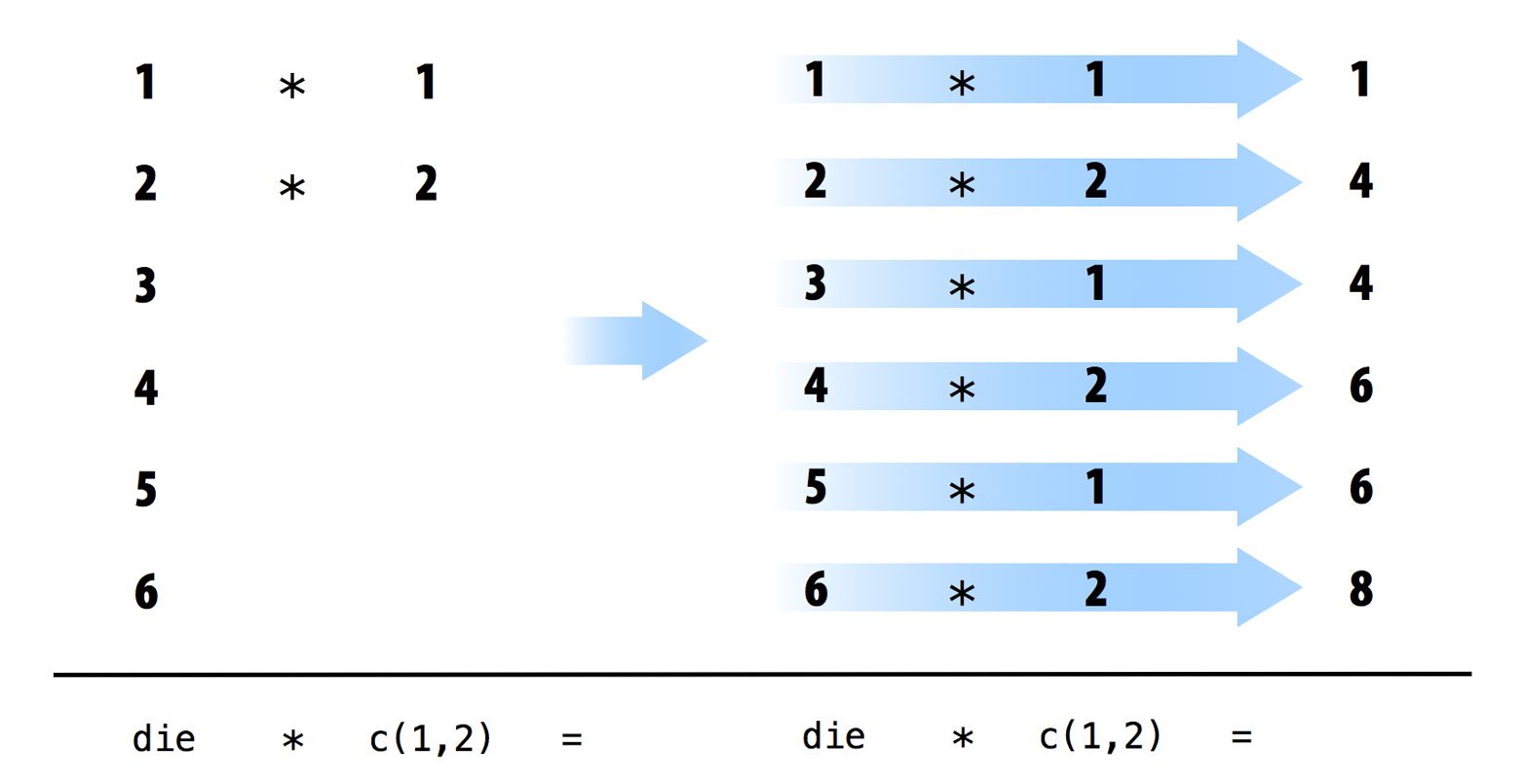
Element-wise operations are a very useful feature in R because they manipulate groups of values in an orderly way. When you start working with data sets, element-wise operations will ensure that values from one observation or case are only paired with values from the same observation or case. Element-wise operations also make it easier to write your own programs and functions in R.
It is important to know that operations with vectors are not the same that you might expect if you are expecting R to perform “matrix” operations. R can do inner multiplication with the %*% operator and outer multiplication with the %o% operator:
Now that you can do math with your die object, let’s look at how you could “roll” it. Rolling your die will require something more sophisticated than basic arithmetic; you’ll need to randomly select one of the die’s values. And for that, you will need a function.
R has many functions and puts them all at our disposal. We can use functions to do simple and sophisticated tasks. For example, we can round a number with the round function, or calculate its factorial with the factorial function. Using a function is pretty simple. Just write the name of the function and then the data you want the function to operate on in parentheses:
The data that you pass into the function is called the function’s argument. The argument can be raw data, an R object, or even the results of another R function. In this last case, R will work from the innermost function to the outermost Figure 4.5.

Returning to our die, we can use the sample function to randomly select one of the die’s values; in other words, the sample function can simulate rolling the die.
The sample function takes two arguments: a vector named x and a number named size. sample will return size elements from the vector:
sample(x = 1:4, size = 2)[1] 1 4To roll your die and get a number back, set x to die and sample one element from it. You’ll get a new (maybe different) number each time you roll it:
Many R functions take multiple arguments that help them do their job. You can give a function as many arguments as you like as long as you separate each argument with a comma.
You may have noticed that I set die and 1 equal to the names of the arguments in sample, x and size. Every argument in every R function has a name. You can specify which data should be assigned to which argument by setting a name equal to data, as in the preceding code. This becomes important as you begin to pass multiple arguments to the same function; names help you avoid passing the wrong data to the wrong argument. However, using names is optional. You will notice that R users do not often use the name of the first argument in a function. So you might see the previous code written as:
sample(die, size = 1)[1] 4Often, the name of the first argument is not very descriptive, and it is usually obvious what the first piece of data refers to anyways.
But how do you know which argument names to use? If you try to use a name that a function does not expect, you will likely get an error:
round(3.1415, corners = 2)
## Error in round(3.1415, corners = 2) : unused argument(s) (corners = 2)
If you’re not sure which names to use with a function, you can look up the function’s arguments with args. To do this, place the name of the function in the parentheses behind args. For example, you can see that the round function takes two arguments, one named x and one named digits:
args(round)function (x, digits = 0, ...)
NULLDid you notice that args shows that the digits argument of round is already set to 0? Frequently, an R function will take optional arguments like digits. These arguments are considered optional because they come with a default value. You can pass a new value to an optional argument if you want, and R will use the default value if you do not. For example, round will round your number to 0 digits past the decimal point by default. To override the default, supply your own value for digits:
round(3.1415)[1] 3round(3.1415, digits = 2)[1] 3.14# pi happens to be a built-in value in R
pi[1] 3.141593round(pi)[1] 3You should write out the names of each argument after the first one or two when you call a function with multiple arguments. Why? First, this will help you and others understand your code. It is usually obvious which argument your first input refers to (and sometimes the second input as well). However, you’d need a large memory to remember the third and fourth arguments of every R function. Second, and more importantly, writing out argument names prevents errors.
If you do not write out the names of your arguments, R will match your values to the arguments in your function by order. For example, in the following code, the first value, die, will be matched to the first argument of sample, which is named x. The next value, 1, will be matched to the next argument, size:
sample(die, 1)[1] 6As you provide more arguments, it becomes more likely that your order and R’s order may not align. As a result, values may get passed to the wrong argument. Argument names prevent this. R will always match a value to its argument name, no matter where it appears in the order of arguments:
sample(size = 1, x = die)[1] 1If you set size = 2, you can almost simulate a pair of dice. Before we run that code, think for a minute why that might be the case. sample will return two numbers, one for each die:
sample(die, size = 2)[1] 1 4I said this “almost” works because this method does something funny. If you use it many times, you’ll notice that the second die never has the same value as the first die, which means you’ll never roll something like a pair of threes or snake eyes. What is going on?
By default, sample builds a sample without replacement. To see what this means, imagine that sample places all of the values of die in a jar or urn. Then imagine that sample reaches into the jar and pulls out values one by one to build its sample. Once a value has been drawn from the jar, sample sets it aside. The value doesn’t go back into the jar, so it cannot be drawn again. So if sample selects a six on its first draw, it will not be able to select a six on the second draw; six is no longer in the jar to be selected. Although sample creates its sample electronically, it follows this seemingly physical behavior.
One side effect of this behavior is that each draw depends on the draws that come before it. In the real world, however, when you roll a pair of dice, each die is independent of the other. If the first die comes up six, it does not prevent the second die from coming up six. In fact, it doesn’t influence the second die in any way whatsoever. You can recreate this behavior in sample by adding the argument replace = TRUE:
sample(die, size = 2, replace = TRUE)[1] 4 2The argument replace = TRUE causes sample to sample with replacement. Our jar example provides a good way to understand the difference between sampling with replacement and without. When sample uses replacement, it draws a value from the jar and records the value. Then it puts the value back into the jar. In other words, sample replaces each value after each draw. As a result, sample may select the same value on the second draw. Each value has a chance of being selected each time. It is as if every draw were the first draw.
Sampling with replacement is an easy way to create independent random samples. Each value in your sample will be a sample of size one that is independent of the other values. This is the correct way to simulate a pair of dice:
sample(die, size = 2, replace = TRUE)[1] 6 4Congratulate yourself; you’ve just run your first simulation in R! You now have a method for simulating the result of rolling a pair of dice. If you want to add up the dice, you can feed your result straight into the sum function:
What would happen if you call dice multiple times? Would R generate a new pair of dice values each time? Let’s give it a try:
dice[1] 1 5dice[1] 1 5dice[1] 1 5The name dice refers to a vector of two numbers. Calling more than once does not change the value. Each time you call dice, R will show you the result of that one time you called sample and saved the output to dice. R won’t rerun sample(die, 2, replace = TRUE) to create a new roll of the dice. Once you save a set of results to an R object, those results do not change.
However, it would be convenient to have an object that can re-roll the dice whenever you call it. You can make such an object by writing your own R function.
To recap, you already have working R code that simulates rolling a pair of dice:
You can retype this code into the console anytime you want to re-roll your dice. However, this is an awkward way to work with the code. It would be easier to use your code if you wrapped it into its own function, which is exactly what we’ll do now. We’re going to write a function named roll that you can use to roll your virtual dice. When you’re finished, the function will work like this: each time you call roll(), R will return the sum of rolling two dice:
roll()
## 8
roll()
## 3
roll()
## 7Functions may seem mysterious or fancy, but they are just another type of R object. Instead of containing data, they contain code. This code is stored in a special format that makes it easy to reuse the code in new situations. You can write your own functions by recreating this format.
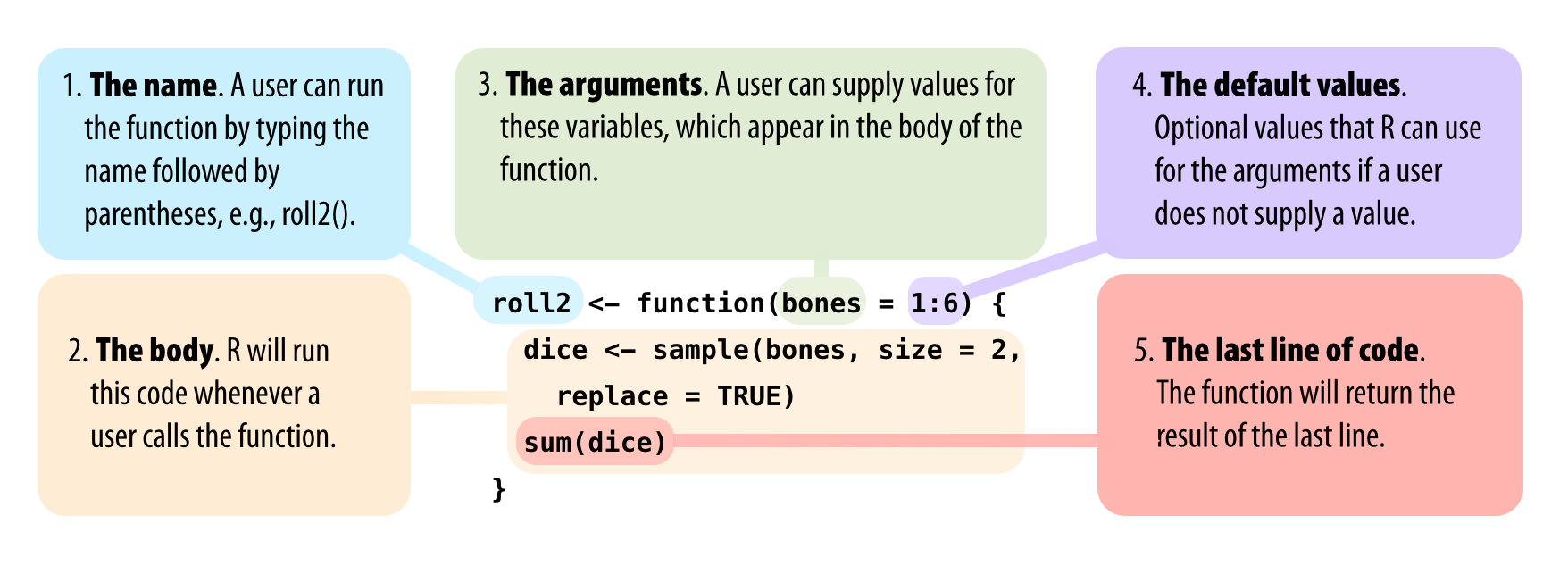
Every function in R has three basic parts: a name, a body of code, and a set of arguments. To make your own function, you need to replicate these parts and store them in an R object, which you can do with the function function. To do this, call function() and follow it with a pair of braces, {}:
my_function <- function() {}This function, as written, doesn’t do anything (yet). However, it is a valid function. You can call it by typing its name followed by an open and closed parenthesis:
my_function()NULLfunction will build a function out of whatever R code you place between the braces. For example, you can turn your dice code into a function by calling:
Notice each line of code between the braces is indented. This makes the code easier to read but has no impact on how the code runs. R ignores spaces and line breaks and executes one complete expression at a time. Note that in other languages like python, spacing is extremely important and part of the language.
Just hit the Enter key between each line after the first brace, {. R will wait for you to type the last brace, }, before it responds.
Don’t forget to save the output of function to an R object. This object will become your new function. To use it, write the object’s name followed by an open and closed parenthesis:
roll()[1] 7You can think of the parentheses as the “trigger” that causes R to run the function. If you type in a function’s name without the parentheses, R will show you the code that is stored inside the function. If you type in the name with the parentheses, R will run that code:
rollfunction ()
{
die <- 1:6
dice <- sample(die, size = 2, replace = TRUE)
sum(dice)
}roll()[1] 4The code that you place inside your function is known as the body of the function. When you run a function in R, R will execute all of the code in the body and then return the result of the last line of code. If the last line of code doesn’t return a value, neither will your function, so you want to ensure that your final line of code returns a value. One way to check this is to think about what would happen if you ran the body of code line by line in the command line. Would R display a result after the last line, or would it not?
Here’s some code that would display a result:
dice
1 + 1
sqrt(2)
And here’s some code that would not:
Again, this is just showing the distinction between expressions and assignments.
What if we removed one line of code from our function and changed the name die to bones (just a name–don’t think of it as important), like this?
Now I’ll get an error when I run the function. The function needs the object bones to do its job, but there is no object named bones to be found (you can check by typing ls() which will show you the names in the environment, or memory).
roll2()
## Error in sample(bones, size = 2, replace = TRUE) :
##   object 'bones' not found
You can supply bones when you call roll2 if you make bones an argument of the function. To do this, put the name bones in the parentheses that follow function when you define roll2:
Now roll2 will work as long as you supply bones when you call the function. You can take advantage of this to roll different types of dice each time you call roll2.
Remember, we’re rolling pairs of dice:
roll2(bones = 1:4)[1] 3roll2(bones = 1:6)[1] 11roll2(1:20)[1] 25Notice that roll2 will still give an error if you do not supply a value for the bones argument when you call roll2:
roll2()
## Error in sample(bones, size = 2, replace = TRUE) :
##   argument "bones" is missing, with no default
You can prevent this error by giving the bones argument a default value. To do this, set bones equal to a value when you define roll2:
Now you can supply a new value for bones if you like, and roll2 will use the default if you do not:
roll2()[1] 6You can give your functions as many arguments as you like. Just list their names, separated by commas, in the parentheses that follow function. When the function is run, R will replace each argument name in the function body with the value that the user supplies for the argument. If the user does not supply a value, R will replace the argument name with the argument’s default value (if you defined one).
To summarize, function helps you construct your own R functions. You create a body of code for your function to run by writing code between the braces that follow function. You create arguments for your function to use by supplying their names in the parentheses that follow function. Finally, you give your function a name by saving its output to an R object, as shown in Figure 4.6.
Once you’ve created your function, R will treat it like every other function in R. Think about how useful this is. Have you ever tried to create a new Excel option and add it to Microsoft’s menu bar? Or a new slide animation and add it to Powerpoint’s options? When you work with a programming language, you can do these types of things. As you learn to program in R, you will be able to create new, customized, reproducible tools for yourself whenever you like.
function to create these parts. Assign the result to a name, so you can call the function later.”
Scripts are code that are saved for later reuse or editing. An R script is just a plain text file that you save R code in. You can open an R script in RStudio by going to File > New File > R script in the menu bar. RStudio will then open a fresh script above your console pane, as shown in Figure 4.7.
I strongly encourage you to write and edit all of your R code in a script before you run it in the console. Why? This habit creates a reproducible record of your work. When you’re finished for the day, you can save your script and then use it to rerun your entire analysis the next day. Scripts are also very handy for editing and proofreading your code, and they make a nice copy of your work to share with others. To save a script, click the scripts pane, and then go to File > Save As in the menu bar.
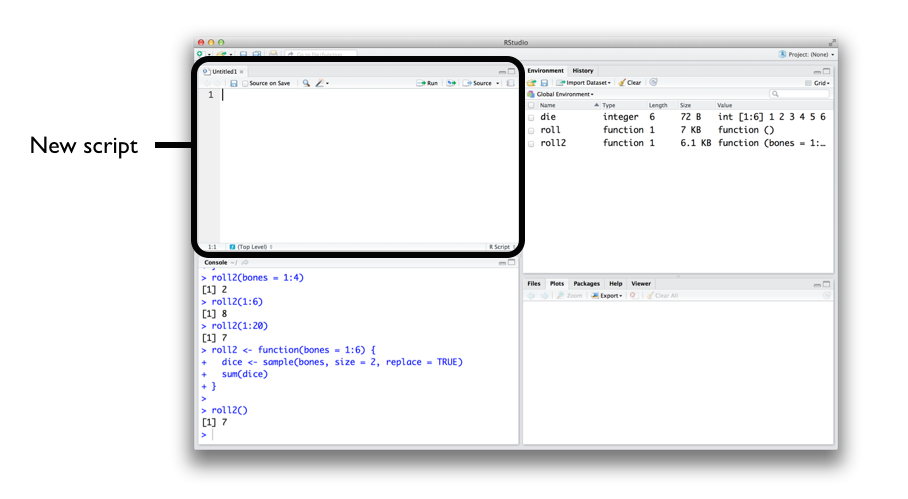
RStudio comes with many built-in features that make it easy to work with scripts. First, you can automatically execute a line of code in a script by clicking the Run button at the top of the editor panel.
R will run whichever line of code your cursor is on. If you have a whole section highlighted, R will run the highlighted code. Alternatively, you can run the entire script by clicking the Source button. Don’t like clicking buttons? You can use Control + Return as a shortcut for the Run button. On Macs, that would be Command + Return.
If you’re not convinced about scripts, you soon will be. It becomes a pain to write multi-line code in the console’s single-line command line. Let’s avoid that headache and open your first script now before we move to the next chapter.
Extract function
RStudio comes with a tool that can help you build functions. To use it, highlight the lines of code in your R script that you want to turn into a function. Then click Code > Extract Function in the menu bar. RStudio will ask you for a function name to use and then wrap your code in a function call. It will scan the code for undefined variables and use these as arguments.
You may want to double-check RStudio’s work. It assumes that your code is correct, so if it does something surprising, you may have a problem in your code.
We’ve covered a lot of ground already. You now have a virtual die stored in your computer’s memory, as well as your own R function that rolls a pair of dice. You’ve also begun speaking the R language.
The two most important components of the R language are objects, which store data, and functions, which manipulate data. R also uses a host of operators like +, -, *, /, and <- to do basic tasks. As a data scientist, you will use R objects to store data in your computer’s memory, and you will use functions to automate tasks and do complicated calculations.