mat1 <- matrix(1:16,nrow=4)
mat1
[,1] [,2] [,3] [,4]
[1,] 1 5 9 13
[2,] 2 6 10 14
[3,] 3 7 11 15
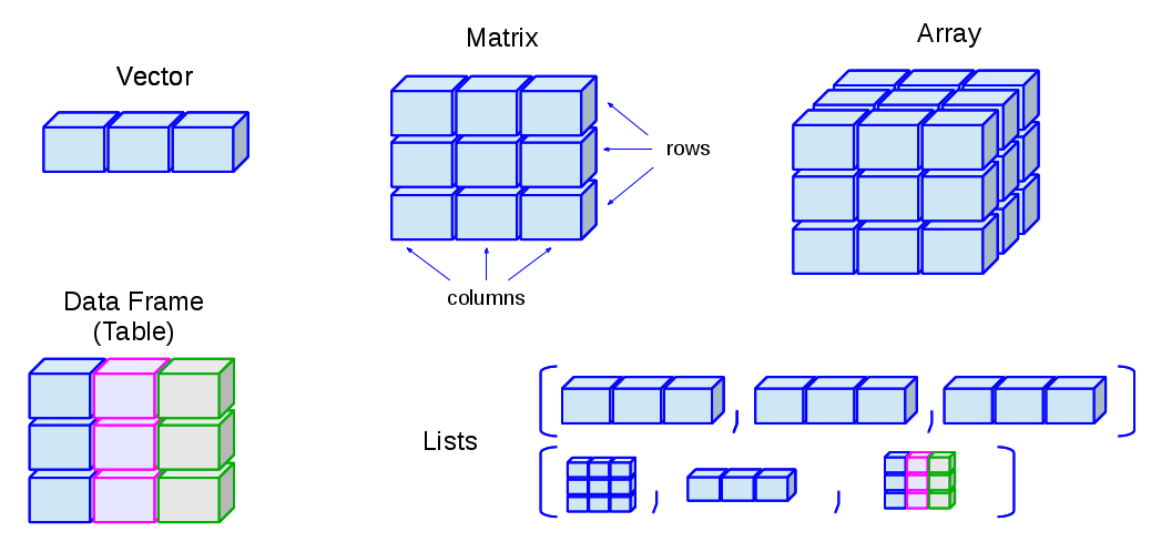
[4,] 4 8 12 16A matrix is a rectangular collection of the same data type (see Figure 9.1). It can be viewed as a collection of column vectors all of the same length and the same type (i.e. numeric, character or logical) OR a collection of row vectors, again all of the same type and length. A data.frame is also a rectangular array. All of the columns must be the same length, but they may be of different types. The rows and columns of a matrix or data frame can be given names. However these are implemented differently in R; many operations will work for one but not both, often a source of confusion.
There are many ways to create a matrix in R. One of the simplest is to use the matrix() function. In the code below, we’ll create a matrix from a vector from 1:16.
mat1 <- matrix(1:16,nrow=4)
mat1 [,1] [,2] [,3] [,4]
[1,] 1 5 9 13
[2,] 2 6 10 14
[3,] 3 7 11 15
[4,] 4 8 12 16The same is possible, but specifying that the matrix be “filled” by row.
mat1 <- matrix(1:16,nrow=4,byrow = TRUE)
mat1
[,1] [,2] [,3] [,4]
[1,] 1 2 3 4
[2,] 5 6 7 8
[3,] 9 10 11 12
[4,] 13 14 15 16Notice the subtle difference in the order that the numbers go into the matrix.
We can also build a matrix from parts by “binding” vectors together:
x <- 1:10
y <- rnorm(10)
Each of the vectors above is of length 10 and both are “numeric”, so we can make them into a matrix. Using rbind binds rows (r) into a matrix.
mat <- rbind(x,y)
mat
[,1] [,2] [,3] [,4] [,5] [,6] [,7]
x 1.0000000 2.0000000 3.0000000 4.0000000 5.0000000 6.000000 7.0000000
y 0.0626442 -0.2605412 0.4941094 0.7590003 -0.3364795 -0.259964 0.6668722
[,8] [,9] [,10]
x 8.0000 9.0000000 10.0000000
y 1.9121 -0.1715687 0.2585426The alternative to rbind is cbind that binds columns (c) together.
mat <- cbind(x,y)
mat
x y
[1,] 1 0.0626442
[2,] 2 -0.2605412
[3,] 3 0.4941094
[4,] 4 0.7590003
[5,] 5 -0.3364795
[6,] 6 -0.2599640
[7,] 7 0.6668722
[8,] 8 1.9120996
[9,] 9 -0.1715687
[10,] 10 0.2585426Inspecting the names associated with rows and columns is often useful, particularly if the names have human meaning.
We can also change the names of the matrix by assigning valid names to the columns or rows.
[1] "apples" "oranges"mat apples oranges
[1,] 1 0.0626442
[2,] 2 -0.2605412
[3,] 3 0.4941094
[4,] 4 0.7590003
[5,] 5 -0.3364795
[6,] 6 -0.2599640
[7,] 7 0.6668722
[8,] 8 1.9120996
[9,] 9 -0.1715687
[10,] 10 0.2585426Matrices have dimensions.
Indexing for matrices works as for vectors except that we now need to include both the row and column (in that order). We can access elements of a matrix using the square bracket [ indexing method. Elements can be accessed as var[r, c]. Here, r and c are vectors describing the elements of the matrix to select.
The indices in R start with one, meaning that the first element of a vector or the first row/column of a matrix is indexed as one.
This is different from some other programming languages, such as Python, which use zero-based indexing, meaning that the first element of a vector or the first row/column of a matrix is indexed as zero.
It is important to be aware of this difference when working with data in R, especially if you are coming from a programming background that uses zero-based indexing. Using the wrong index can lead to unexpected results or errors in your code.
# The 2nd element of the 1st row of mat
mat[1,2]
oranges
0.0626442 # The first ROW of mat
mat[1,] apples oranges
1.0000000 0.0626442 # The first COLUMN of mat
mat[,1] [1] 1 2 3 4 5 6 7 8 9 10# and all elements of mat that are > 4; note no comma
mat[mat>4][1] 5 6 7 8 9 10## [1] 5 6 7 8 9 10Note that in the last case, there is no “,”, so R treats the matrix as a long vector (length=20). This is convenient, sometimes, but it can also be a source of error, as some code may “work” but be doing something unexpected.
We can also use indexing to exclude a row or column by prefixing the selection with a - sign.
mat[,-1] # remove first column [1] 0.0626442 -0.2605412 0.4941094 0.7590003 -0.3364795 -0.2599640
[7] 0.6668722 1.9120996 -0.1715687 0.2585426mat[-c(1:5),] # remove first five rows apples oranges
[1,] 6 -0.2599640
[2,] 7 0.6668722
[3,] 8 1.9120996
[4,] 9 -0.1715687
[5,] 10 0.2585426We can create a matrix filled with random values drawn from a normal distribution for our work below.
       V1                 V2
 Min.   :-1.33238   Min.   :-1.48278
 1st Qu.:-0.52761   1st Qu.:-0.68838
 Median : 0.31448   Median :-0.14225
 Mean   :-0.01296   Mean   :-0.06669
 3rd Qu.: 0.35305   3rd Qu.: 0.79620
 Max.   : 0.66566   Max.   : 1.03073
Multiplication and division works similarly to vectors. When multiplying by a vector, for example, the values of the vector are reused. In the simplest case, let’s multiply the matrix by a constant (vector of length 1).
# multiply all values in the matrix by 20
m2 = m*20
summary(m2)
V1 V2
Min. :-26.6476 Min. :-29.656
1st Qu.:-10.5523 1st Qu.:-13.768
Median : 6.2896 Median : -2.845
Mean : -0.2592 Mean : -1.334
3rd Qu.: 7.0609 3rd Qu.: 15.924
Max. : 13.3133 Max. : 20.615 By combining subsetting with assignment, we can make changes to just part of a matrix.
# and add 100 to the first column of m
m2[,1] = m2[,1] + 100
# summarize m
summary(m2)
V1 V2
Min. : 73.35 Min. :-29.656
1st Qu.: 89.45 1st Qu.:-13.768
Median :106.29 Median : -2.845
Mean : 99.74 Mean : -1.334
3rd Qu.:107.06 3rd Qu.: 15.924
Max. :113.31 Max. : 20.615 A somewhat common transformation for a matrix is to transpose which changes rows to columns. One might need to do this if an assay output from a lab machine puts samples in rows and genes in columns, for example, while in Bioconductor/R, we often want the samples in columns and the genes in rows.
t(m2) [,1] [,2] [,3] [,4] [,5] [,6] [,7]
[1,] 106.815460 86.01827 85.80517 73.35238 106.11582 99.73604 106.46335
[2,] 4.638628 16.99678 18.68817 -14.44571 -10.32864 -29.65564 -11.73298
[,8] [,9] [,10]
[1,] 112.64556 107.14273 113.31326
[2,] 12.70564 20.61456 -20.81924Again, we just need a matrix to play with. We’ll use rnorm again, but with a slight twist.
Since these data are from a normal distribution, we can look at a row (or column) to see what the mean and standard deviation are.
mean(m3[,1])[1] 5.104862sd(m3[,1])[1] 1.521707# or a row
mean(m3[1,])[1] 5.708435sd(m3[1,])[1] 2.126164There are some useful convenience functions for computing means and sums of data in all of the columns and rows of matrices.
colMeans(m3) [1] 5.104862 5.067118 4.674373 5.207726 6.422428 5.276819 4.127895 5.238015
[9] 5.501107 4.458434rowMeans(m3) [1] 5.708435 5.500776 5.496619 4.886450 4.969435 5.826565 3.985788 5.264617
[9] 4.918903 4.521188rowSums(m3) [1] 57.08435 55.00776 54.96619 48.86450 49.69435 58.26565 39.85788 52.64617
[9] 49.18903 45.21188colSums(m3) [1] 51.04862 50.67118 46.74373 52.07726 64.22428 52.76819 41.27895 52.38015
[9] 55.01107 44.58434We can look at the distribution of column means:
   Min. 1st Qu.  Median    Mean 3rd Qu.    Max.
  4.128   4.773   5.156   5.108   5.267   6.422
Note that this is centered pretty closely around the selected mean of 5 above.
How about the standard deviation? There is not a colSd function, but it turns out that we can easily apply functions that take vectors as input, like sd and “apply” them across either the rows (the first dimension) or columns (the second) dimension.
   Min. 1st Qu.  Median    Mean 3rd Qu.    Max.
  1.417   1.882   2.004   2.155   2.450   3.329
Again, take a look at the distribution which is centered quite close to the selected standard deviation when we created our matrix.
For this set of exercises, we are going to rely on a dataset that comes with R. It gives the number of sunspots per month from 1749-1983. The dataset comes as a ts or time series data type which I convert to a matrix using the following code.
Just run the code as is and focus on the rest of the exercises.
data(sunspots)
sunspot_mat <- matrix(as.vector(sunspots),ncol=12,byrow = TRUE)
colnames(sunspot_mat) <- as.character(1:12)
rownames(sunspot_mat) <- as.character(1749:1983)After the conversion above, what does sunspot_mat look like? Use functions to find the number of rows, the number of columns, the class, and some basic summary statistics.
Practice subsetting the matrix a bit by selecting:
sunspot_mat[1:10,]
sunspot_mat[,7]
sunspot_mat['1979',7]
These next few exercises take advantage of the fact that calling a univariate statistical function (one that expects a vector) works for matrices by just making a vector of all the values in the matrix. What is the highest (max) number of sunspots recorded in these data?
max(sunspot_mat)And the minimum?
min(sunspot_mat)And the overall mean and median?
Use the hist() function to look at the distribution of all the monthly sunspot data.
hist(sunspot_mat)Read about the breaks argument to hist() to try to increase the number of breaks in the histogram to increase the resolution slightly. Adjust your hist() and breaks to your liking.
hist(sunspot_mat, breaks=40)Now, let’s move on to summarizing the data a bit to learn about the pattern of sunspots varies by month or by year. Examine the dataset again. What do the columns represent? And the rows?
# just a quick glimpse of the data will give us a sense
head(sunspot_mat)
We’d like to look at the distribution of sunspots by month. How can we do that?
Assign the month summary above to a variable and summarize it to get a sense of the spread over months.
Play the same game for years to get the per-year mean?
Make a plot of the yearly means. Do you see a pattern?