2  The R language

In this chapter, we’re going to get an introduction to the R language, so we can dive right into programming. We’re going to create a pair of virtual dice that can generate random numbers. No need to worry if you’re new to programming. We’ll return to many of the concepts here in more detail later.

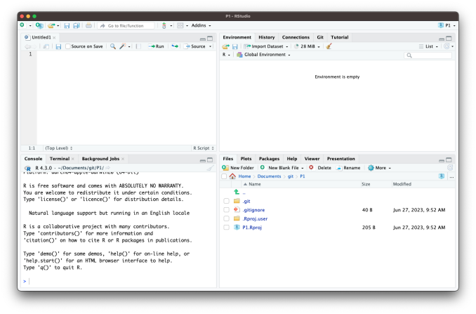
To simulate a pair of dice, we need to break down each die into its essential features. A die can only show one of six numbers: 1, 2, 3, 4, 5, and 6. We can capture the die’s essential characteristics by saving these numbers as a group of values in the computer. Let’s save these numbers first and then figure out a way to “roll” our virtual die.

2.1 The R User Interface

The RStudio interface is simple. You type R code into the bottom line of the RStudio console pane and then click Enter to run it. The code you type is called a command, because it will command your computer to do something for you. The line you type it into is called the command line.

Figure 2.1: Your computer does your bidding when you type R commands at the prompt in the bottom line of the console pane. Don’t forget to hit the Enter key. When you first open RStudio, the console appears in the pane on your left, but you can change this with File > Tools > Global Options in the menu bar.

When you type a command at the prompt and hit Enter, your computer executes the command and shows you the results. Then RStudio displays a fresh prompt for your next command. For example, if you type 1 + 1 and hit Enter, RStudio will display:

> 1 + 1
[1] 2
>

You’ll notice that a [1] appears next to your result. R is just letting you know that this line begins with the first value in your result. Some commands return more than one value, and their results may fill up multiple lines. For example, the command 100:130 returns 31 values; it creates a sequence of integers from 100 to 130. Notice that new bracketed numbers appear at the start of the second and third lines of output. These numbers just mean that the second line begins with the 14th value in the result, and the third line begins with the 25th value. You can mostly ignore the numbers that appear in brackets:

> 100:130
 [1] 100 101 102 103 104 105 106 107 108 109 110 111 112
[14] 113 114 115 116 117 118 119 120 121 122 123 124 125
[25] 126 127 128 129 130

Tip

The colon operator (:) returns every integer between two integers. It is an easy way to create a sequence of numbers.

When do we compile?

In some languages, like C, Java, and FORTRAN, you have to compile your human-readable code into machine-readable code (often 1s and 0s) before you can run it. If you’ve programmed in such a language before, you may wonder whether you have to compile your R code before you can use it. The answer is no. R is a dynamic programming language, which means R automatically interprets your code as you run it.

If you type an incomplete command and press Enter, R will display a + prompt, which means R is waiting for you to type the rest of your command. Either finish the command or hit Escape to start over:

> 5 -
+
+ 1
[1] 4

If you type a command that R doesn’t recognize, R will return an error message. If you ever see an error message, don’t panic. R is just telling you that your computer couldn’t understand or do what you asked it to do. You can then try a different command at the next prompt:

> 3 % 5
Error: unexpected input in "3 % 5"
>

Tip

Whenever you get an error message in R, consider googling the error message. You’ll often find that someone else has had the same problem and has posted a solution online. Simply cutting-and-pasting the error message into a search engine will often work

Once you get the hang of the command line, you can easily do anything in R that you would do with a calculator. For example, you could do some basic arithmetic:

2 * 3   

[1] 6

4 - 1   

[1] 3

# this obeys order-of-operations
6 / (4 - 1)   

[1] 2

Most of the arithmetic operators in R are the same as those on a calculator, but R uses different symbols for some of them:

• Addition: +
• Subtraction: -
• Multiplication: *
• Division: /
• Exponentiation: ^
• Modulo: %%

The ^ operator raises the number to its left to the power of the number to its right: for example 3^2 is 9. The modulo returns the remainder of the division of the number to the left by the number on its right, for example 5 modulo 3 or 5 %% 3 is 2.

Tip

R treats the hashtag character, #, in a special way; R will not run anything that follows a hashtag on a line. This makes hashtags very useful for adding comments and annotations to your code. Humans will be able to read the comments, but your computer will pass over them. The hashtag is known as the commenting symbol in R.

Cancelling commands

Some R commands may take a long time to run. You can cancel a command once it has begun by pressing ctrl + c or by clicking the “stop sign” if it is available in Rstudio. Note that it may also take R a long time to cancel the command.

2.1.1 An exercise

That’s the basic interface for executing R code in RStudio. Think you have it? If so, try doing these simple tasks. If you execute everything correctly, you should end up with the same number that you started with:

1. Choose any number and add 2 to it.
2. Multiply the result by 3.
3. Subtract 6 from the answer.
4. Divide what you get by 3.

10 + 2

[1] 12

12 * 3

[1] 36

36 - 6

[1] 30

30 / 3

[1] 10

2.2 Objects

Now that you know how to use R, let’s use it to make a virtual die. The : operator from a couple of pages ago gives you a nice way to create a group of numbers from one to six. The : operator returns its results as a vector (we are going to work with vectors in more detail), a one-dimensional set of numbers:

1:6
## 1 2 3 4 5 6

That’s all there is to how a virtual die looks! But you are not done yet. Running 1:6 generated a vector of numbers for you to see, but it didn’t save that vector anywhere for later use. If we want to use those numbers again, we’ll have to ask your computer to save them somewhere. You can do that by creating an R object.

R lets you save data by storing it inside an R object. What is an object? Just a name that you can use to call up stored data. For example, you can save data into an object like a or b. Wherever R encounters the object, it will replace it with the data saved inside, like so:

a <- 1
a

[1] 1

a + 2

[1] 3

What just happened?

1. To create an R object, choose a name and then use the less-than symbol, <, followed by a minus sign, -, to save data into it. This combination looks like an arrow, <-. R will make an object, give it your name, and store in it whatever follows the arrow. So a <- 1 stores 1 in an object named a.
2. When you ask R what’s in a, R tells you on the next line.
3. You can use your object in new R commands, too. Since a previously stored the value of 1, you’re now adding 1 to 2.

Assignment vs expressions

Everything that you type into the R console can be assigned to one of two categories:

• Assignments
• Expressions

An expression is a command that tells R to do something. For example, 1 + 2 is an expression that tells R to add 1 and 2. When you type an expression into the R console, R will evaluate the expression and return the result. For example, if you type 1 + 2 into the R console, R will return 3. Expressions can have “side effects” but they don’t explicitly result in anything being added to R memory.

5 + 2

[1] 7

28 %% 3

[1] 1

3^2

[1] 9

5 + 4 * 4 + 4 ^ 4 / 10

[1] 46.6

While using R as a calculator is interesting, to do useful and interesting things, we need to assign values to objects. To create objects, we need to give it a name followed by the assignment operator <- (or, entirely equivalently, =) and the value we want to give it:

weight_kg <- 55

So, for another example, the following code would create an object named die that contains the numbers one through six. To see what is stored in an object, just type the object’s name by itself:

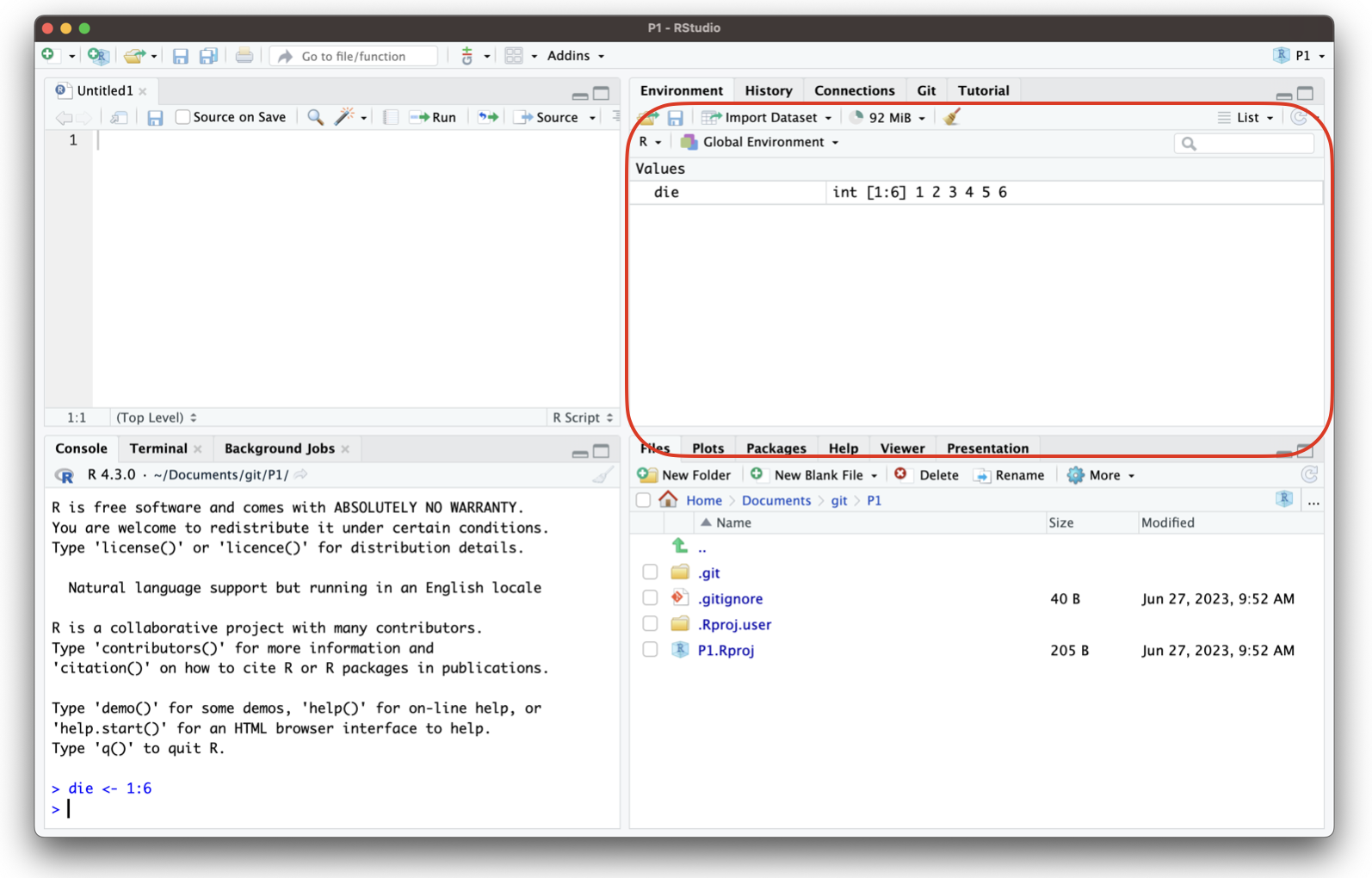
die <- 1:6
die

[1] 1 2 3 4 5 6

When you create an object, the object will appear in the environment pane of RStudio, as shown in Figure 2.2. This pane will show you all of the objects you’ve created since opening RStudio.

Figure 2.2: Assignment creates an object in the environment pane.

You can name an object in R almost anything you want, but there are a few rules. First, a name cannot start with a number. Second, a name cannot use some special symbols, like ^, !, $, @, +, -, /, or *:

Good names	Names that cause errors
a	1trial
b	$
FOO	^mean
my_var	2nd
.day	!bad

Capitalization matters

R is case-sensitive, so name and Name will refer to different objects:

> Name = 0
> Name + 1
[1] 1
> name + 1
Error: object 'name' not found

The error above is a common one!

Finally, R will overwrite any previous information stored in an object without asking you for permission. So, it is a good idea to not use names that are already taken:

my_number <- 1
my_number 

[1] 1

my_number <- 999
my_number

[1] 999

You can see which object names you have already used with the function ls:

ls()

Your environment will contain different names than mine, because you have probably created different objects.

You can also see which names you have used by examining RStudio’s environment pane.

We can remove an object from the environment using the rm function. For example, to create and then remove an object named to_disappear, you could run the following code:

to_disappear <- 1
rm(to_disappear)
to_disappear # this will return an error

We now have a virtual die that is stored in the computer’s memory and which has a name that we can use to refer to it. You can access it whenever you like by typing the word die.

So what can you do with this die? Quite a lot. R will replace an object with its contents whenever the object’s name appears in a command. So, for example, you can do all sorts of math with the die. Math isn’t so helpful for rolling dice, but manipulating sets of numbers will be your stock and trade as a data scientist. So let’s take a look at how to do that:

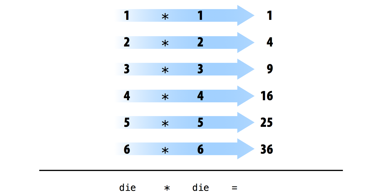
die - 1

[1] 0 1 2 3 4 5

die / 2

[1] 0.5 1.0 1.5 2.0 2.5 3.0

die * die

[1]  1  4  9 16 25 36

R uses element-wise execution when working with a vector like die. When you manipulate a set of numbers, R will apply the same operation to each element in the set. So for example, when you run die - 1, R subtracts one from each element of die.

When you use two or more vectors in an operation, R will line up the vectors and perform a sequence of individual operations. For example, when you run die * die, R lines up the two die vectors and then multiplies the first element of vector 1 by the first element of vector 2. R then multiplies the second element of vector 1 by the second element of vector 2, and so on, until every element has been multiplied. The result will be a new vector the same length as the first two {Figure 2.3}.

Figure 2.3: “When R performs element-wise execution, it matches up vectors and then manipulates each pair of elements independently.”

If you give R two vectors of unequal lengths, R will repeat the shorter vector until it is as long as the longer vector, and then do the math, as shown in Figure 2.4. This isn’t a permanent change–the shorter vector will be its original size after R does the math. If the length of the short vector does not divide evenly into the length of the long vector, R will return a warning message. This behavior is known as vector recycling, and it helps R do element-wise operations:

1:2

[1] 1 2

1:4

[1] 1 2 3 4

die

[1] 1 2 3 4 5 6

die + 1:2

[1] 2 4 4 6 6 8

die + 1:4

Warning in die + 1:4: longer object length is not a multiple of shorter object
length

[1] 2 4 6 8 6 8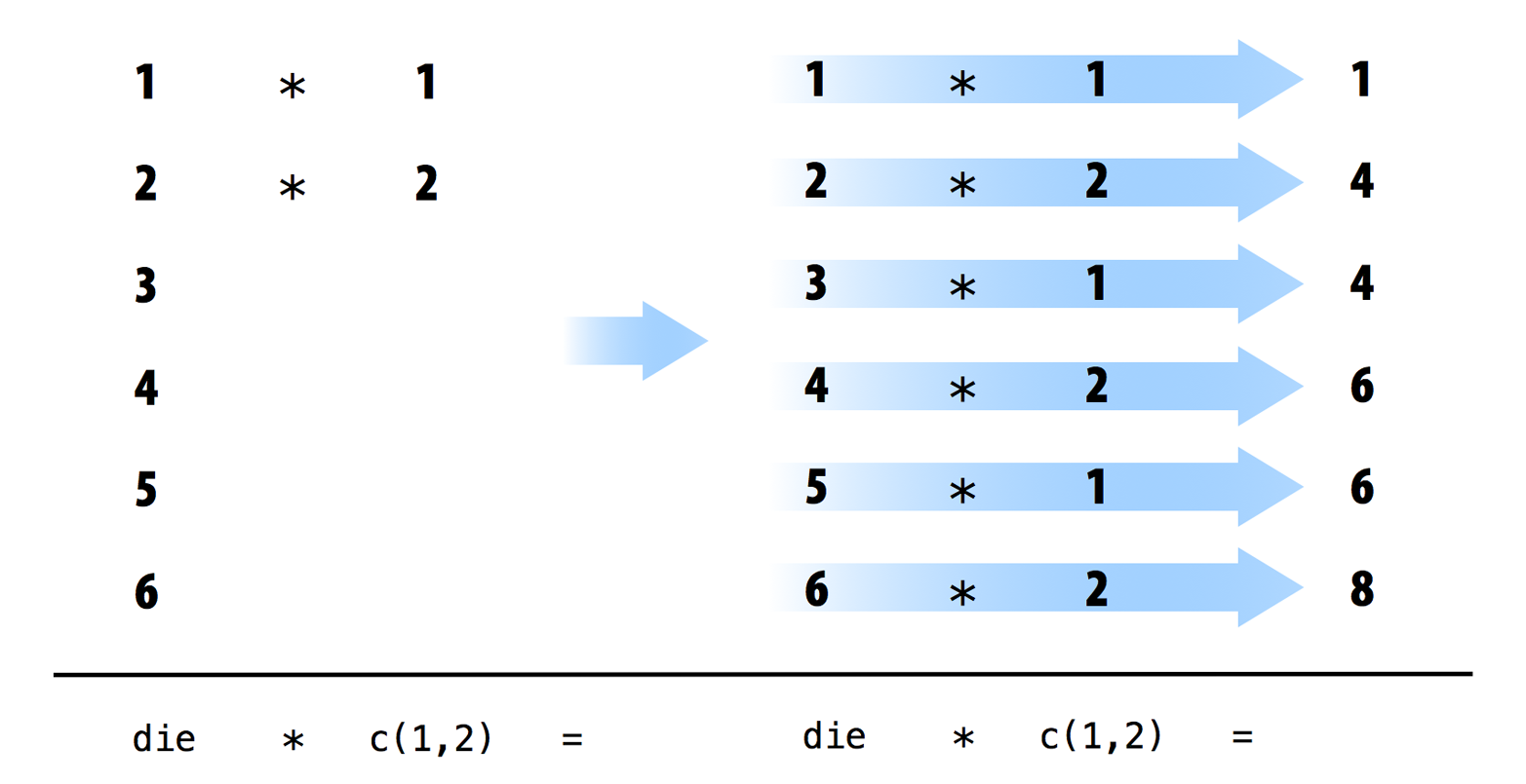

Figure 2.4: “R will repeat a short vector to do element-wise operations with two vectors of uneven lengths.”

Element-wise operations are a very useful feature in R because they manipulate groups of values in an orderly way. When you start working with data sets, element-wise operations will ensure that values from one observation or case are only paired with values from the same observation or case. Element-wise operations also make it easier to write your own programs and functions in R.

Element-wise operations are not matrix operations

It is important to know that operations with vectors are not the same that you might expect if you are expecting R to perform “matrix” operations. R can do inner multiplication with the %*% operator and outer multiplication with the %o% operator:

# Inner product (1*1 + 2*2 + 3*3 + 4*4 + 5*5 + 6*6)
die %*% die
# Outer product (will be a 6 x 6 matrix with 
#  all possible products of the two vectors)
die %o% die

Now that you can do math with your die object, let’s look at how you could “roll” it. Rolling your die will require something more sophisticated than basic arithmetic; you’ll need to randomly select one of the die’s values. And for that, you will need a function.

While we’ve seen functions already, the next section will discuss R functions more formally.

3 Up and Running with R

The only meaningful way of interacting with R is by typing into the R console. At the most basic level, anything that we type at the command line will fall into one of two categories:

1. Assignments

   x = 1
   y <- 2

2. Expressions

   1 + pi + sin(42)

   [1] 3.225071

The assignment type is obvious because either the The <- or = are used. Note that when we type expressions, R will return a result. In this case, the result of R evaluating 1 + pi + sin(42) is 3.2250711.

The standard R prompt is a “>” sign. When present, R is waiting for the next expression or assignment. If a line is not a complete R command, R will continue the next line with a “+”. For example, typing the fillowing with a “Return” after the second “+” will result in R giving back a “+” on the next line, a prompt to keep typing.

1 + pi +
sin(3.7)

[1] 3.611757