round(3.1415)[1] 3factorial(3)[1] 6In the previous chapter, you learned about storing data in R objects. Now, we’ll explore R functions. Functions let you save and reuse code. They’re very useful because you can write code once and use it repeatedly. You can also share your functions with others. This chapter will show you how to create functions to simulate rolling two dice.
You can recognize that you are using a function in R when you see a name followed by parentheses. For example, mean(1:6) is a function call. The name of the function is mean, and the data that the function is operating on is 1:6. Functions are a fundamental part of R. They are used to perform simple and complex tasks.
The functions that we use in R come from a variety of sources. Some functions are built into R, and others are part of packages that you can install. You can also write your own functions. A major strength of R is that it is open-source, which means that anyone can write and share functions. This has led to a large and diverse collection of functions that you can use in your work.
R has many functions that others have written and it puts them all at our disposal. We can use functions to do simple and sophisticated tasks. For example, we can round a number with the round function, or calculate its factorial with the factorial function. Using a function is pretty simple. Just write the name of the function and then the data you want the function to operate on in parentheses.
The data that you pass into the function is called the function’s argument. The argument can be raw data, an R object, or even the results of another R function. In this last case, R will work from the innermost function to the outermost Figure 3.1.
Recall that we had a die object that we used to simulate rolling a die:
die <- 1:6We can use that object as input to functions, just like we can use raw data. For example, we can calculate the mean of the die:

Returning to our die, we can use the sample function to randomly select one of the die’s values; in other words, the sample function can simulate rolling the die.
The sample function takes two arguments: a vector named x and a number named size. sample will return size elements from the vector:
sample(x = 1:4, size = 2)[1] 2 3To roll your die and get a number back, set x to die and sample one element from it. You’ll get a new (maybe different) number each time you roll it:
Many R functions take multiple arguments that help them do their job. You can give a function as many arguments as you like as long as you separate each argument with a comma.
You may have noticed that I set die and 1 equal to the names of the arguments in sample, x and size. Every argument in every R function has a name. You can specify which data should be assigned to which argument by setting a name equal to data, as in the preceding code. This becomes important as you begin to pass multiple arguments to the same function; names help you avoid passing the wrong data to the wrong argument. However, using names is optional. You will notice that R users do not often use the name of the first argument in a function. So you might see the previous code written as:
sample(die, size = 1)[1] 3Often, the name of the first argument is not very descriptive, and it is usually obvious what the first piece of data refers to anyways.
But how do you know which argument names to use? If you try to use a name that a function does not expect, you will likely get an error:
round(3.1415, corners = 2)
## Error in round(3.1415, corners = 2) : unused argument(s) (corners = 2)
If you’re not sure which names to use with a function, you can look up the function’s arguments with args. To do this, place the name of the function in the parentheses behind args. For example, you can see that the round function takes two arguments, one named x and one named digits:
args(round)function (x, digits = 0, ...)
NULLDid you notice that args shows that the digits argument of round is already set to 0? Frequently, an R function will take optional arguments like digits. These arguments are considered optional because they come with a default value. You can pass a new value to an optional argument if you want, and R will use the default value if you do not. For example, round will round your number to 0 digits past the decimal point by default. To override the default, supply your own value for digits:
round(3.1415)[1] 3round(3.1415, digits = 2)[1] 3.14# pi happens to be a built-in value in R
pi[1] 3.141593round(pi)[1] 3help
When you are using a function that is new to you, consider looking up the help() for that function. You can do this by typing ? followed by the function’s name. For example, to look up the sample function, type ?sample. This will open a help page that describes the function and its arguments. You can also look up the help page for a function by typing help(sample). The help page will show you the names of the function’s arguments and their default values, as well as examples of how to use the function.
You should write out the names of each argument after the first one or two when you call a function with multiple arguments. Why? First, this will help you and others understand your code. It is usually obvious which argument your first input refers to (and sometimes the second input as well). However, you’d need a large memory to remember the third and fourth arguments of every R function. Second, and more importantly, writing out argument names prevents errors.
If you do not write out the names of your arguments, R will match your values to the arguments in your function by order. For example, in the following code, the first value, die, will be matched to the first argument of sample, which is named x. The next value, 1, will be matched to the next argument, size:
sample(die, 1)[1] 3As you provide more arguments, it becomes more likely that your order and R’s order may not align. As a result, values may get passed to the wrong argument. Argument names prevent this. R will always match a value to its argument name, no matter where it appears in the order of arguments:
sample(size = 1, x = die)[1] 6If you set size = 2, you can almost simulate a pair of dice. Before we run that code, think for a minute why that might be the case. sample will return two numbers, one for each die:
sample(die, size = 2)[1] 2 4I said this “almost” works because this method does something funny. If you use it many times, you’ll notice that the second die never has the same value as the first die, which means you’ll never roll something like a pair of threes or snake eyes. What is going on?
By default, sample builds a sample without replacement. To see what this means, imagine that sample places all of the values of die in a jar or urn. Then imagine that sample reaches into the jar and pulls out values one by one to build its sample. Once a value has been drawn from the jar, sample sets it aside. The value doesn’t go back into the jar, so it cannot be drawn again. So if sample selects a six on its first draw, it will not be able to select a six on the second draw; six is no longer in the jar to be selected. Although sample creates its sample electronically, it follows this seemingly physical behavior.
One side effect of this behavior is that each draw depends on the draws that come before it. In the real world, however, when you roll a pair of dice, each die is independent of the other. If the first die comes up six, it does not prevent the second die from coming up six. In fact, it doesn’t influence the second die in any way whatsoever. You can recreate this behavior in sample by adding the argument replace = TRUE:
sample(die, size = 2, replace = TRUE)[1] 6 3The argument replace = TRUE causes sample to sample with replacement. Our jar example provides a good way to understand the difference between sampling with replacement and without. When sample uses replacement, it draws a value from the jar and records the value. Then it puts the value back into the jar. In other words, sample replaces each value after each draw. As a result, sample may select the same value on the second draw. Each value has a chance of being selected each time. It is as if every draw were the first draw.
Sampling with replacement is an easy way to create independent random samples. Each value in your sample will be a sample of size one that is independent of the other values. This is the correct way to simulate a pair of dice:
sample(die, size = 2, replace = TRUE)[1] 1 5Congratulate yourself; you’ve just run your first simulation in R! You now have a method for simulating the result of rolling a pair of dice. If you want to add up the dice, you can feed your result straight into the sum function:
What would happen if you call dice multiple times? Would R generate a new pair of dice values each time? Let’s give it a try:
dice[1] 4 5dice[1] 4 5dice[1] 4 5The name dice refers to a vector of two numbers. Calling more than once does not change the favlue. Each time you call dice, R will show you the result of that one time you called sample and saved the output to dice. R won’t rerun sample(die, 2, replace = TRUE) to create a new roll of the dice. Once you save a set of results to an R object, those results do not change.
However, it would be convenient to have an object that can re-roll the dice whenever you call it. You can make such an object by writing your own R function.
To recap, you already have working R code that simulates rolling a pair of dice:
You can retype this code into the console anytime you want to re-roll your dice. However, this is an awkward way to work with the code. It would be easier to use your code if you wrapped it into its own function, which is exactly what we’ll do now. We’re going to write a function named roll that you can use to roll your virtual dice. When you’re finished, the function will work like this: each time you call roll(), R will return the sum of rolling two dice:
roll()
## 8
roll()
## 3
roll()
## 7Functions may seem mysterious or fancy, but they are just another type of R object. Instead of containing data, they contain code. This code is stored in a special format that makes it easy to reuse the code in new situations. You can write your own functions by recreating this format.
Every function in R has three basic parts: a name, a body of code, and a set of arguments. To make your own function, you need to replicate these parts and store them in an R object, which you can do with the function function. To do this, call function() and follow it with a pair of braces, {}:
my_function <- function() {}This function, as written, doesn’t do anything (yet). However, it is a valid function. You can call it by typing its name followed by an open and closed parenthesis:
my_function()NULLfunction will build a function out of whatever R code you place between the braces. For example, you can turn your dice code into a function by calling:
Notice each line of code between the braces is indented. This makes the code easier to read but has no impact on how the code runs. R ignores spaces and line breaks and executes one complete expression at a time. Note that in other languages like python, spacing is extremely important and part of the language.
Just hit the Enter key between each line after the first brace, {. R will wait for you to type the last brace, }, before it responds.
Don’t forget to save the output of function to an R object. This object will become your new function. To use it, write the object’s name followed by an open and closed parenthesis:
roll()[1] 7You can think of the parentheses as the “trigger” that causes R to run the function. If you type in a function’s name without the parentheses, R will show you the code that is stored inside the function. If you type in the name with the parentheses, R will run that code:
rollfunction() {
die <- 1:6
dice <- sample(die, size = 2, replace = TRUE)
sum(dice)
}roll()[1] 8The code that you place inside your function is known as the body of the function. When you run a function in R, R will execute all of the code in the body and then return the result of the last line of code. If the last line of code doesn’t return a value, neither will your function, so you want to ensure that your final line of code returns a value. One way to check this is to think about what would happen if you ran the body of code line by line in the command line. Would R display a result after the last line, or would it not?
Here’s some code that would display a result:
dice
1 + 1
sqrt(2)
And here’s some code that would not:
Again, this is just showing the distinction between expressions and assignments.
What if we removed one line of code from our function and changed the name die to bones (just a name–don’t think of it as important), like this?
Now I’ll get an error when I run the function. The function needs the object bones to do its job, but there is no object named bones to be found (you can check by typing ls() which will show you the names in the environment, or memory).
roll2()
## Error in sample(bones, size = 2, replace = TRUE) :
##   object 'bones' not found
You can supply bones when you call roll2 if you make bones an argument of the function. To do this, put the name bones in the parentheses that follow function when you define roll2:
Now roll2 will work as long as you supply bones when you call the function. You can take advantage of this to roll different types of dice each time you call roll2.
Remember, we’re rolling pairs of dice:
roll2(bones = 1:4)[1] 7roll2(bones = 1:6)[1] 8roll2(1:20)[1] 22Notice that roll2 will still give an error if you do not supply a value for the bones argument when you call roll2:
roll2()
## Error in sample(bones, size = 2, replace = TRUE) :
##   argument "bones" is missing, with no default
You can prevent this error by giving the bones argument a default value. To do this, set bones equal to a value when you define roll2:
Now you can supply a new value for bones if you like, and roll2 will use the default if you do not:
roll2()[1] 5You can give your functions as many arguments as you like. Just list their names, separated by commas, in the parentheses that follow function. When the function is run, R will replace each argument name in the function body with the value that the user supplies for the argument. If the user does not supply a value, R will replace the argument name with the argument’s default value (if you defined one).
To summarize, function helps you construct your own R functions. You create a body of code for your function to run by writing code between the braces that follow function. You create arguments for your function to use by supplying their names in the parentheses that follow function. Finally, you give your function a name by saving its output to an R object, as shown in Figure 3.2.
Once you’ve created your function, R will treat it like every other function in R. Think about how useful this is. Have you ever tried to create a new Excel option and add it to Microsoft’s menu bar? Or a new slide animation and add it to Powerpoint’s options? When you work with a programming language, you can do these types of things. As you learn to program in R, you will be able to create new, customized, reproducible tools for yourself whenever you like.
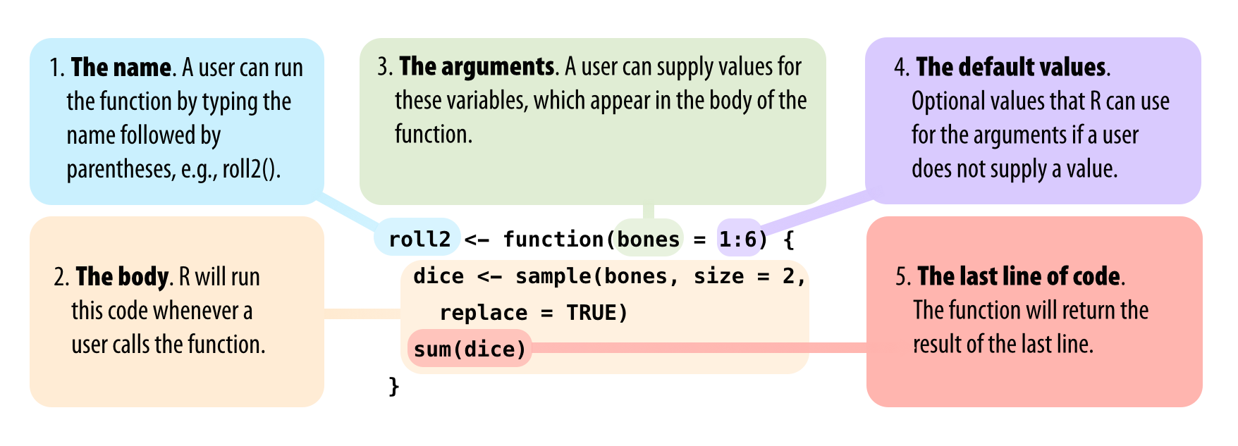
function to create these parts. Assign the result to a name, so you can call the function later.”