10  Data Frames

While R has many different data types, the one that is central to much of the power and popularity of R is the data.frame. A data.frame looks a bit like an R matrix in that it has two dimensions, rows and columns. However, data.frames are usually viewed as a set of columns representing variables and the rows representing the values of those variables. Importantly, a data.frame may contain different data types in each of its columns; matrices must contain only one data type. This distinction is important to remember, as there are specific approaches to working with R data.frames that may be different than those for working with matrices.

10.1 Dataset

The insurance dataset is described in the book Machine Learning with R by Brett Lantz. The dataset describes medical information and costs billed by health insurance companies for 1338 individuals in 2013, as compiled by the United States Census Bureau.

Variables include:

• age

  age of primary beneficiary

• sex

  insurance contractor gender, female, male

• bmi

  Body mass index, providing an understanding of body, weights that are relatively high or low relative to height, objective index of body weight (kg / m ^ 2) using the ratio of height to weight, ideally 18.5 to 24.9

• children

  Number of children covered by health insurance / Number of dependents

• smoker

  Smoking status

• region

  the beneficiary’s residential area in the US, northeast, southeast, southwest, northwest.

• charges

  Individual medical costs billed by health insurance

We will load the data directly from the web, but you can also download the data from the link at github¹.

¹ Insurance data csv file, https://raw.githubusercontent.com/stedy/Machine-Learning-with-R-datasets/master/insurance.csv

insurance_url <- "https://raw.githubusercontent.com/stedy/Machine-Learning-with-R-datasets/master/insurance.csv"
insurance <- read.csv(insurance_url)

Explore the dataset a bit to understand its structure and contents. For example, you can use the head() function to view the first few rows of the dataset.

head(insurance)

  age    sex    bmi children smoker    region   charges
1  19 female 27.900        0    yes southwest 16884.924
2  18   male 33.770        1     no southeast  1725.552
3  28   male 33.000        3     no southeast  4449.462
4  33   male 22.705        0     no northwest 21984.471
5  32   male 28.880        0     no northwest  3866.855
6  31 female 25.740        0     no southeast  3756.622

And you can examine the dimensions of the dataset using the dim(), which returns the number of rows and columns in the dataset, the ncol() function, which returns the number of columns, and the nrow() function, which returns the number of rows.

dim(insurance)

[1] 1338    7

ncol(insurance)

[1] 7

nrow(insurance)

[1] 1338

Note that with the dim() function, the number of rows is given first, followed by the number of columns.

Notice that, while the BMI variable represents a measure of a person’s weight relative to their height, there is no discrete variable for whether a person is obese or not. The World Health Organization (WHO) defines obesity as a BMI greater than or equal to 30. We can create a new variable, obese, that indicates whether a person is obese based on their BMI.

insurance$obese <- ifelse(insurance$bmi >= 30, "obese", "not obese")

If we examine the dataset again, we can see that the new variable obese has been added to the dataset.

head(insurance)

  age    sex    bmi children smoker    region   charges     obese
1  19 female 27.900        0    yes southwest 16884.924 not obese
2  18   male 33.770        1     no southeast  1725.552     obese
3  28   male 33.000        3     no southeast  4449.462     obese
4  33   male 22.705        0     no northwest 21984.471 not obese
5  32   male 28.880        0     no northwest  3866.855 not obese
6  31 female 25.740        0     no southeast  3756.622 not obese

10.2 Inspecting data.frames

There are a few functions that are useful for inspecting the contents of a data.frame:

• Overviews of content
  • head() to show first few rows
  • tail() to show last few rows
• Size
  • dim() for dimensions (rows, columns)
  • nrow()
  • ncol()
  • object.size() for power users interested in the memory used to store an object
• Data and attribute summaries
  • colnames() to get the names of the columns
  • rownames() to get the “names” of the rows–may not be present
  • summary() to get per-column summaries of the data in the data.frame.

# Show the first few rows
head(insurance)

  age    sex    bmi children smoker    region   charges     obese
1  19 female 27.900        0    yes southwest 16884.924 not obese
2  18   male 33.770        1     no southeast  1725.552     obese
3  28   male 33.000        3     no southeast  4449.462     obese
4  33   male 22.705        0     no northwest 21984.471 not obese
5  32   male 28.880        0     no northwest  3866.855 not obese
6  31 female 25.740        0     no southeast  3756.622 not obese

# Show the last few rows
tail(insurance)

     age    sex   bmi children smoker    region   charges     obese
1333  52 female 44.70        3     no southwest 11411.685     obese
1334  50   male 30.97        3     no northwest 10600.548     obese
1335  18 female 31.92        0     no northeast  2205.981     obese
1336  18 female 36.85        0     no southeast  1629.833     obese
1337  21 female 25.80        0     no southwest  2007.945 not obese
1338  61 female 29.07        0    yes northwest 29141.360 not obese

# Get the dimensions of the data.frame
dim(insurance)

[1] 1338    8

# Get the number of rows and columns
nrow(insurance)

[1] 1338

ncol(insurance)

[1] 8

# Get the names of the columns
colnames(insurance)

[1] "age"      "sex"      "bmi"      "children" "smoker"   "region"   "charges" 
[8] "obese"   

# Basic summary of the data
summary(insurance)

      age            sex                 bmi           children    
 Min.   :18.00   Length:1338        Min.   :15.96   Min.   :0.000  
 1st Qu.:27.00   Class :character   1st Qu.:26.30   1st Qu.:0.000  
 Median :39.00   Mode  :character   Median :30.40   Median :1.000  
 Mean   :39.21                      Mean   :30.66   Mean   :1.095  
 3rd Qu.:51.00                      3rd Qu.:34.69   3rd Qu.:2.000  
 Max.   :64.00                      Max.   :53.13   Max.   :5.000  
    smoker             region             charges         obese          
 Length:1338        Length:1338        Min.   : 1122   Length:1338       
 Class :character   Class :character   1st Qu.: 4740   Class :character  
 Mode  :character   Mode  :character   Median : 9382   Mode  :character  
                                       Mean   :13270                     
                                       3rd Qu.:16640                     
                                       Max.   :63770                     

In RStudio, there is an additional function, View() (note the capital “V”) that opens the first 1000 rows (default) in the RStudio window, akin to a spreadsheet view.

View(insurance)

10.3 Accessing variables (columns) and subsetting

In R, data.frames can be subset similarly to other two-dimensional data structures. The [ in R is used to denote subsetting of any kind. When working with two-dimensional data, we need two values inside the [ ] to specify the details. The specification is [rows, columns]. For example, to get the first three rows of insurance, use:

insurance[1:3, ]

  age    sex   bmi children smoker    region   charges     obese
1  19 female 27.90        0    yes southwest 16884.924 not obese
2  18   male 33.77        1     no southeast  1725.552     obese
3  28   male 33.00        3     no southeast  4449.462     obese

Note how the second number, the columns, is blank. R takes that to mean “all the columns”. Similarly, we can combine rows and columns specification arbitrarily.

insurance[1:3, 1:3]

  age    sex   bmi
1  19 female 27.90
2  18   male 33.77
3  28   male 33.00

Because selecting a single variable, or column, is such a common operation, there are two shortcuts for doing so with data.frames. The first, the $ operator works like so:

# Look at the column names, just to refresh memory
colnames(insurance)

[1] "age"      "sex"      "bmi"      "children" "smoker"   "region"   "charges" 
[8] "obese"   

# Note that I am using "head" here to limit the output
head(insurance$age)

[1] 19 18 28 33 32 31

# What is the actual length of "symbol"?
length(insurance$age)

[1] 1338

The second is related to the fact that, in R, data.frames are also lists. We subset a list by using [[]] notation. To get the second column of insurance, we can use:

head(insurance[[2]])

[1] "female" "male"   "male"   "male"   "male"   "female"

Alternatively, we can use the column name:

head(insurance[["age"]])

[1] 19 18 28 33 32 31

10.3.1 Some data exploration

There are a couple of columns that include numeric values. Which columns are numeric?

class(insurance$age)

[1] "integer"

class(insurance$obese)

[1] "character"

class(insurance$children)

[1] "integer"

library(gridExtra)
library(grid)
library(dplyr)

Attaching package: 'dplyr'

The following object is masked from 'package:gridExtra':

    combine

The following objects are masked from 'package:stats':

    filter, lag

The following objects are masked from 'package:base':

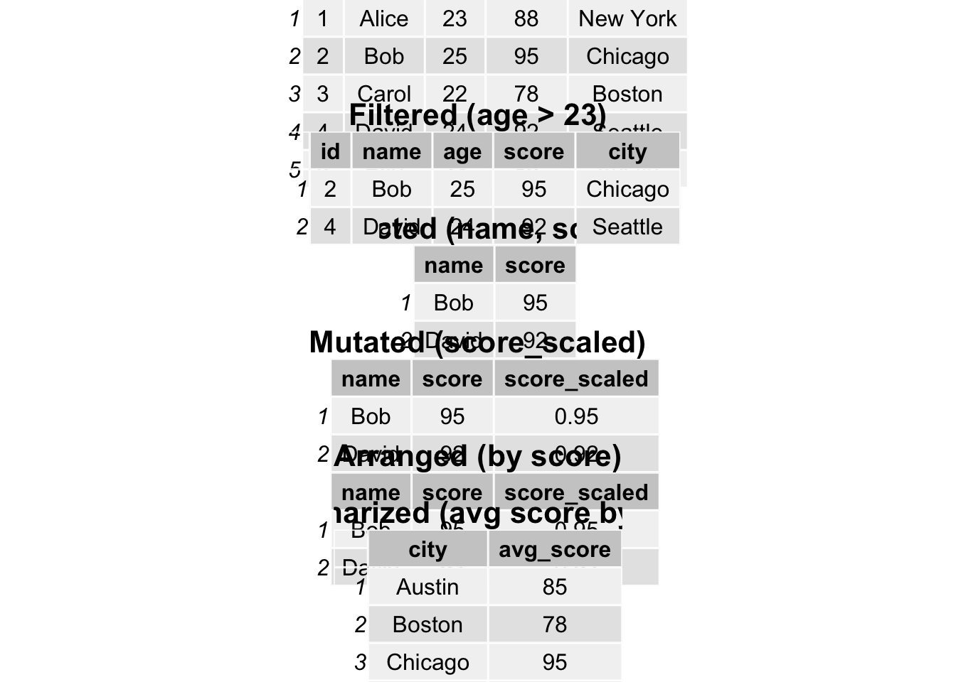
    intersect, setdiff, setequal, union

# Original DataFrame
df <- data.frame(
    id = c(1, 2, 3, 4, 5),
    name = c("Alice", "Bob", "Carol", "David", "Eve"),
    age = c(23, 25, 22, 24, 23),
    score = c(88, 95, 78, 92, 85),
    city = c("New York", "Chicago", "Boston", "Seattle", "Austin")
)

# Filter
df_filtered <- df %>% filter(age > 23)

# Select
df_selected <- df_filtered %>% select(name, score)

# Mutate
df_mutated <- df_selected %>% mutate(score_scaled = score / 100)

# Arrange
df_arranged <- df_mutated %>% arrange(desc(score))

# Summarize
df_grouped <- df %>%
    group_by(city) %>%
    summarize(avg_score = mean(score))

# Function to create table grobs
create_table_grob <- function(df, title) {
    table_grob <- tableGrob(df)
    title_grob <- textGrob(title, gp = gpar(fontsize = 16, fontface = "bold"))
    padding <- unit(0.5, "line")
    table_grob <- gtable::gtable_add_rows(table_grob, heights = grobHeight(title_grob) + padding, pos = 0)
    table_grob <- gtable::gtable_add_grob(table_grob, list(title_grob), 1, 1, 1, ncol(table_grob))
    table_grob
}

# Creating table grobs
original_grob <- create_table_grob(df, "Original DataFrame")
filtered_grob <- create_table_grob(df_filtered, "Filtered (age > 23)")
selected_grob <- create_table_grob(df_selected, "Selected (name, score)")
mutated_grob <- create_table_grob(df_mutated, "Mutated (score_scaled)")
arranged_grob <- create_table_grob(df_arranged, "Arranged (by score)")
summarized_grob <- create_table_grob(df_grouped, "Summarized (avg score by city)")

# Arrange tables in a grid
grid.arrange(
    original_grob, filtered_grob,
    selected_grob, mutated_grob,
    arranged_grob, summarized_grob,
    nrow = 6
)