Chapter 6 Visualizing geographic data without maps
You may have seen visualizations of COVID-19 cases plotted on a map. These maps often represent quantitative information either using color in proportion to values (these are called “choropleths”) or circle area proportional to values (these are called bubble plots). While visually striking, these maps are limited in terms of the amount of quantitative information they can communicate about regions. Here, we take a different approach that allows us to create basically any visual display of quantitative information and present it with an approximation of the geographic context.
library(dplyr)
library(tidyr)
library(purrr)
library(ggplot2)
library(zoo)
library(plotly)
library(geofacet)
library(sars2pack)
6.1 Prepping the data from sars2pack
Let’s start with US county-level data from JHU and state-level data from the COVID Tracking Project.
## Rows: 2,291,240
## Columns: 15
## $ UID          <dbl> 84001001, 84001001, 84001001, 84001001, 84001001, 840010…
## $ iso2         <chr> "US", "US", "US", "US", "US", "US", "US", "US", "US", "U…
## $ iso3         <chr> "USA", "USA", "USA", "USA", "USA", "USA", "USA", "USA", …
## $ code3        <dbl> 840, 840, 840, 840, 840, 840, 840, 840, 840, 840, 840, 8…
## $ fips         <chr> "01001", "01001", "01001", "01001", "01001", "01001", "0…
## $ county       <chr> "Autauga", "Autauga", "Autauga", "Autauga", "Autauga", "…
## $ state        <chr> "Alabama", "Alabama", "Alabama", "Alabama", "Alabama", "…
## $ country      <chr> "US", "US", "US", "US", "US", "US", "US", "US", "US", "U…
## $ Lat          <dbl> 32.53953, 32.53953, 32.53953, 32.53953, 32.53953, 32.539…
## $ Long         <dbl> -86.64408, -86.64408, -86.64408, -86.64408, -86.64408, -…
## $ Combined_Key <chr> "Autauga, Alabama, US", "Autauga, Alabama, US", "Autauga…
## $ Population   <dbl> NA, NA, NA, NA, NA, NA, NA, NA, NA, NA, NA, NA, NA, NA, …
## $ date         <date> 2020-01-22, 2020-01-23, 2020-01-24, 2020-01-25, 2020-01…
## $ count        <dbl> 0, 0, 0, 0, 0, 0, 0, 0, 0, 0, 0, 0, 0, 0, 0, 0, 0, 0, 0,…
## $ subset <chr> "confirmed", "confirmed", "confirmed", "confirmed", "con…## Rows: 16,931
## Columns: 16
## $ date <date> 2020-12-29, 2020-12-29, 2020-12-29, 2020-12-2…
## $ fips <chr> "00002", "00001", "00005", "00060", "00004", "…
## $ state <chr> "AK", "AL", "AR", "AS", "AZ", "CA", "CO", "CT"…
## $ positive <int> 44581, 351804, 219246, 0, 507222, 2187221, 328…
## $ negative <int> 1215264, 1571253, 1841869, 2140, 2310576, 3018…
## $ death <int> 201, 4737, 3603, 0, 8640, 24526, 4687, 5924, 7…
## $ pending <int> NA, NA, NA, NA, NA, NA, NA, NA, NA, NA, 6925, …
## $ hospitalized <int> 1004, 33452, 11168, NA, 36075, NA, 18230, 1225…
## $ hospitalizedCurrently <int> 83, 2804, 1161, NA, 4475, 21240, 1188, 1226, 2…
## $ recovered <int> 7165, 193149, 194436, NA, 74223, NA, 17652, 98…
## $ inIcuCumulative <int> NA, 2424, NA, NA, NA, NA, NA, NA, NA, NA, NA, …
## $ inIcuCurrently <int> NA, NA, 382, NA, 1053, 4390, NA, NA, 72, 60, N…
## $ onVentilatorCurrently <int> 10, NA, 198, NA, 720, NA, NA, NA, 35, NA, NA, …
## $ onVentilatorCumulative <int> NA, 1394, 1199, NA, NA, NA, NA, NA, NA, NA, NA…
## $ dateChecked <dttm> 2020-12-29 03:59:00, 2020-12-29 11:00:00, 202…
## $ dataQualityGrade <chr> "A", "A", "A+", "D", "A+", "B", "A", "B", "A+"…We need to very lightly clean cumulative data that should be monotonically increasing day-over-day (but isn’t always) and convert it from cumulative values to daily incidents. The data are in different formats, so we’ll use slightly different data munging workflows.
The JHU data don’t contain a value for every location-date-subset combination, so we need to fill in those gaps.
iusa <- cusa %>%
  arrange(Combined_Key, subset, date) %>%
  group_by(Combined_Key, subset) %>%
  mutate(count = pmin.int(count, dplyr::lead(count, order_by = date), na.rm = TRUE),
         incidents =  pmax.int(pmap_dbl(list(count, -1*dplyr::lag(count, order_by = date)),
                                        ~ sum(..., na.rm = TRUE)),
                               0, na.rm = TRUE)) %>%
  ungroup() %>%
  complete(date, subset,
           nesting(UID, iso2, iso3, code3, fips, county, state, country, Lat, Long, Combined_Key),
           fill = list(incidents = 0)) %>%
  replace_na(list(incidents = 0)) %>%
  group_by(Combined_Key, subset) %>%
  arrange(date) %>%
  mutate(ma7 = rollmean(incidents, k = 7, fill = NA, align = "right")) %>%
  ungroup() %>%
  filter(date >= "2020-03-15", iso2 == "US")

glimpse(iusa)
## Rows: 2,060,740
## Columns: 17
## $ date <date> 2020-03-15, 2020-03-15, 2020-03-15, 2020-03-15, 2020-03…
## $ subset <chr> "confirmed", "confirmed", "confirmed", "confirmed", "con…
## $ UID <dbl> 84001001, 84001003, 84001005, 84001007, 84001009, 840010…
## $ iso2 <chr> "US", "US", "US", "US", "US", "US", "US", "US", "US", "U…
## $ iso3 <chr> "USA", "USA", "USA", "USA", "USA", "USA", "USA", "USA", …
## $ code3 <dbl> 840, 840, 840, 840, 840, 840, 840, 840, 840, 840, 840, 8…
## $ fips <chr> "01001", "01003", "01005", "01007", "01009", "01011", "0…
## $ county <chr> "Autauga", "Baldwin", "Barbour", "Bibb", "Blount", "Bull…
## $ state <chr> "Alabama", "Alabama", "Alabama", "Alabama", "Alabama", "…
## $ country <chr> "US", "US", "US", "US", "US", "US", "US", "US", "US", "U…
## $ Lat <dbl> 32.53953, 30.72775, 31.86826, 32.99642, 33.98211, 32.100…
## $ Long <dbl> -86.64408, -87.72207, -85.38713, -87.12511, -86.56791, -…
## $ Combined_Key <chr> "Autauga, Alabama, US", "Baldwin, Alabama, US", "Barbour…
## $ Population <dbl> NA, NA, NA, NA, NA, NA, NA, NA, NA, NA, NA, NA, NA, NA, …
## $ count <dbl> 0, 1, 0, 0, 0, 0, 0, 0, 0, 0, 0, 0, 0, 0, 0, 0, 0, 0, 0,…
## $ incidents <dbl> 0, 1, 0, 0, 0, 0, 0, 0, 0, 0, 0, 0, 0, 0, 0, 0, 0, 0, 0,…
## $ ma7 <dbl> 0.0000000, 0.1428571, 0.0000000, 0.0000000, 0.0000000, 0…The COVID Tracking Project data doesn’t have a record for every location-date combination and can contain NA values, so we need to fill in the gaps and also transform it into long format for plotting
US_states <- c('AL', 'AK', 'AR', 'AZ', 'CA', 'CO', 'CT', 'DC', 'DE', 'FL', 'GA',
               'HI', 'IA', 'ID', 'IL', 'IN', 'KS', 'KY' ,'LA', 'MA', 'MD', 'ME',
               'MI', 'MN', 'MO', 'MS', 'MT', 'NC', 'ND', 'NE', 'NH', 'NJ', 'NM',
               'NV', 'NY', 'OH', 'OK', 'OR', 'PA', 'RI', 'SC', 'SD', 'TN', 'TX',
               'UT', 'VA', 'VT', 'WA', 'WI', 'WV', 'WY')

ictp <- ctp %>%
  group_by(state) %>%
  mutate_at(c("positive", "negative", "death"), ~ pmin.int(., dplyr::lead(., order_by = date), na.rm = TRUE)) %>%
  mutate_at(c("positive", "negative", "death"),
            list(incidents = ~ pmax.int(pmap_dbl(list(., -1*dplyr::lag(., order_by = date)),
                                           ~ sum(..., na.rm = TRUE)),
                                  0, na.rm = TRUE))) %>%
  complete(date, nesting(state, fips),
           fill = list(positive_incidents = 0, negative_incidents = 0, death_incidents = 0)) %>%
  mutate(test_incidents = pmap_dbl(list(positive_incidents, negative_incidents), ~ sum(..., na.rm = TRUE)),
         pos_pct = positive_incidents / test_incidents) %>%
  replace_na(list(positive = 0, negative = 0, death = 0)) %>%
  arrange(date) %>%
  mutate_at(vars(ends_with("_incidents")), list(ma7 = ~ rollmean(., k = 7, fill = NA, align = "right"))) %>%
  mutate_at(vars(ends_with("_incidents")), na_if, 0) %>%
  mutate(positive_pct_ma7 = positive_incidents_ma7 / test_incidents_ma7) %>%
  ungroup() %>%
  filter(date >= "2020-03-15", state %in% US_states)

glimpse(ictp)
## Rows: 14,790
## Columns: 26
## $ date <date> 2020-03-15, 2020-03-15, 2020-03-15, 2020-03-1…
## $ state <chr> "AK", "AL", "AR", "AZ", "CA", "CO", "CT", "DC"…
## $ fips <chr> "00002", "00001", "00005", "00004", "00006", "…
## $ positive <dbl> 0, 12, 16, 12, 293, 131, 20, 16, 6, 91, 99, 2,…
## $ negative <dbl> 144, 28, 103, 121, 916, 627, 125, 79, 36, 678,…
## $ death <dbl> 0, 0, 0, 0, 5, 1, 0, 0, 0, 4, 1, 0, 0, 0, 0, 0…
## $ pending <int> NA, 46, 30, 50, NA, NA, NA, 20, 32, 454, NA, N…
## $ hospitalized <int> 1, NA, NA, 36, NA, NA, NA, NA, NA, NA, NA, NA,…
## $ hospitalizedCurrently <int> NA, NA, NA, NA, NA, NA, NA, NA, NA, NA, NA, NA…
## $ recovered <int> NA, NA, NA, NA, NA, NA, NA, NA, NA, NA, NA, NA…
## $ inIcuCumulative <int> NA, NA, NA, NA, NA, NA, NA, NA, NA, NA, NA, NA…
## $ inIcuCurrently <int> NA, NA, NA, NA, NA, NA, NA, NA, NA, NA, NA, NA…
## $ onVentilatorCurrently <int> NA, NA, NA, NA, NA, NA, NA, NA, NA, NA, NA, NA…
## $ onVentilatorCumulative <int> NA, NA, NA, NA, NA, NA, NA, NA, NA, NA, NA, NA…
## $ dateChecked <dttm> 2020-03-13 16:30:00, 2020-03-15 14:12:00, 202…
## $ dataQualityGrade <chr> NA, NA, NA, NA, NA, NA, NA, NA, NA, NA, NA, NA…
## $ positive_incidents <dbl> NA, 6, 4, NA, 41, NA, 9, 6, NA, 40, 33, NA, 1,…
## $ negative_incidents <dbl> NA, 6, 38, NA, NA, NA, NA, 30, NA, 200, NA, NA…
## $ death_incidents <dbl> NA, NA, NA, NA, NA, NA, NA, NA, NA, 1, NA, NA,…
## $ test_incidents <dbl> NA, 12, 42, NA, 41, NA, 9, 36, NA, 240, 33, NA…
## $ pos_pct <dbl> NaN, 0.50000000, 0.09523810, NaN, 1.00000000, …
## $ positive_incidents_ma7 <dbl> 0.0000000, 1.7142857, 2.2857143, 1.0000000, 29…
## $ negative_incidents_ma7 <dbl> 18.571429, 4.000000, 13.857143, 11.000000, 64.…
## $ death_incidents_ma7 <dbl> 0.0000000, 0.0000000, 0.0000000, 0.0000000, 0.…
## $ test_incidents_ma7 <dbl> 18.5714286, 5.7142857, 16.1428571, 12.0000000,…
## $ positive_pct_ma7 <dbl> 0.00000000, 0.30000000, 0.14159292, 0.08333333…6.2 Plotting one geographic unit (example: New York state)
Before plotting, let’s customize the theme so we don’t have to do so repeatedly for ever plot.
theme_light2 <-  theme_light() +
  theme(panel.border = element_blank(),
        panel.grid.major.x = element_blank(),
        panel.grid.minor = element_blank(),
        axis.text.x = element_text(angle = -90),
        strip.background = element_blank(),
        strip.text = element_text(color = "black"),
        legend.position = "bottom")
Let’s start by plotting confirmed positive cases and deaths in a single state. As you can see by the vertical bars, these data are fairly noisy. We also know that under-reporting is common around weekends. To address both of these issues, we include a line for rolling 7-day means. To facilitate interpretation, we include another line for the proportion of positive tests. Confirmed positive cases and COVID-19 deaths depend on testing–with insufficient tests, these numbers are under-counted. Heuristically, when 10% or fewer tests return positive, testing is considered sufficient.
g <- ictp %>%
  filter(state == "NY") %>%
  ggplot(aes(x = date))

g +
  geom_col(aes(y = positive_incidents, fill = "positive_incidents"), width = 1, alpha = .5) +
  geom_col(aes(y = death_incidents, fill = "death_incidents"), width = 1, alpha = .7) +
  geom_line(aes(y = positive_incidents_ma7, color = "positive_incidents"), size = 1.5) +
  geom_line(aes(y = death_incidents_ma7, color = "death_incidents"), size = 1.5) +
  geom_line(aes(y = (1000*10)^positive_pct_ma7, color = "pos_pct_ma7"), size = 1.5) +
  scale_y_continuous(trans = scales::pseudo_log_trans(base = 10),
                     name = "Incidents (log 10 scale)", breaks = c(0, 10, 100, 1000, 10000),
                     sec.axis = sec_axis(~log(., base = (1000*10)), breaks = seq(.1, .9, .2),
                                         name = "Positive Test Rate (%, 7-day moving average)")) +
  scale_fill_viridis_d() +
  scale_color_viridis_d() +
  guides(alpha = "none", fill = "none") +
  theme_light2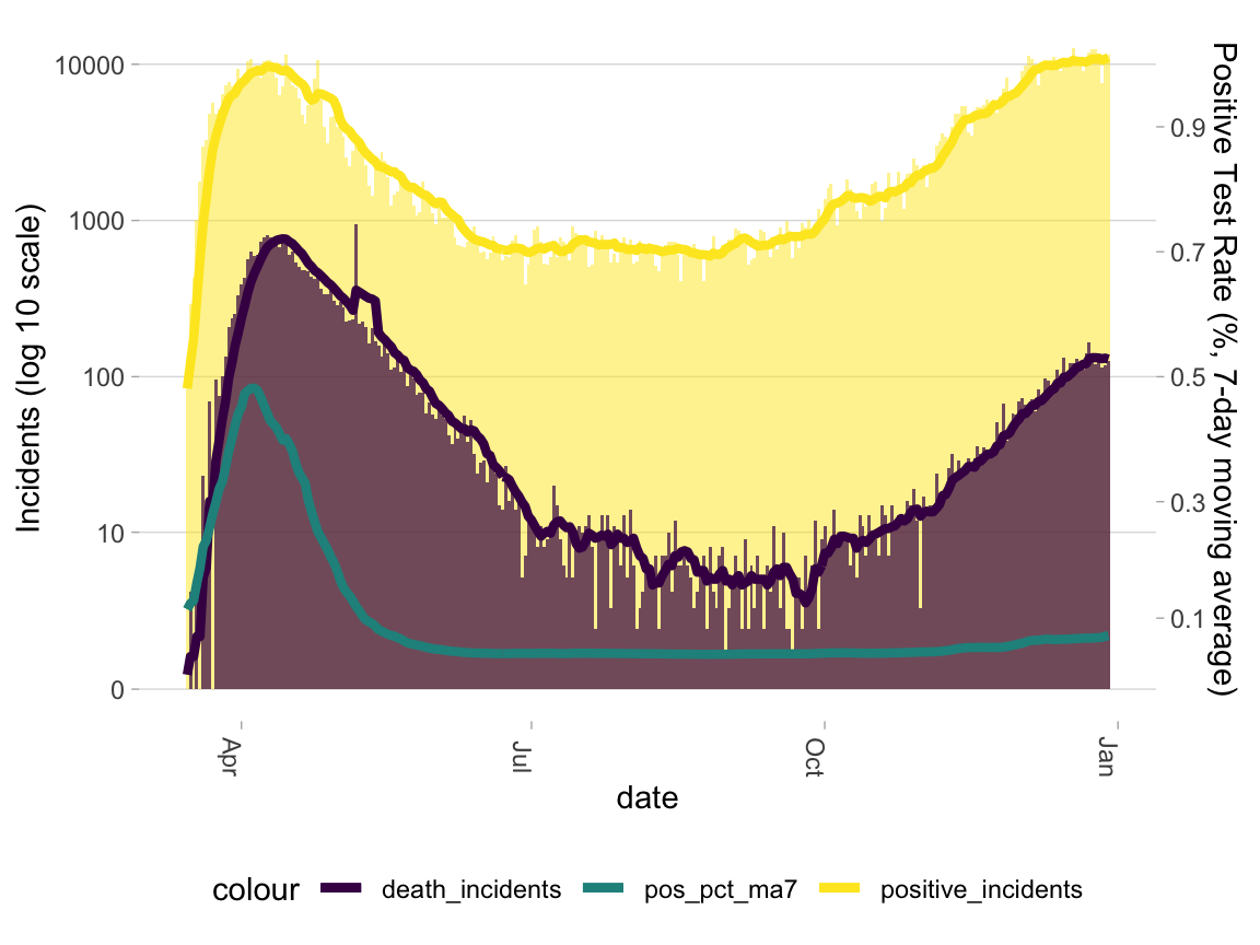
6.3 Plotting multiple geographic units (example: all US states)
Now let’s plot all US states (and DC) simultaneously. To situate these states in their approximate geographic context, we use the {geofacet} package. This package provides a convenient way to arrange small multiples in a grid that correspond to their relative geographic positions. Because these small multiples have less area than the single-state plot, we don’t include daily incidents and instead focus only on 7-day rolling averages.
g_state <- ictp %>%
  ggplot(aes(x = date))

g_state +
  geom_line(aes(y = positive_incidents, color = "positive_incidents"), alpha = 0) +
  geom_line(aes(y = death_incidents, color = "death_incidents"), alpha = 0) +
  geom_area(aes(y = positive_incidents_ma7, fill = "positive_incidents"), alpha = .75) +
  geom_area(aes(y = death_incidents_ma7, fill = "death_incidents"), alpha = .8) +
  geom_line(aes(y = (1000*10)^positive_pct_ma7, color = "pos_pct_ma7")) +
  scale_y_continuous(trans = scales::pseudo_log_trans(base = 10),
                     name = "Incidents (7-day moving average, log 10 scale)", breaks = c(0, 10, 100, 1000, 10000),
                     sec.axis = sec_axis(~log(., base = (1000*10)), breaks = seq(.1, .9, .2),
                                         name = "Positive Test Rate (%, 7-day moving average)")) +
  scale_fill_viridis_d() +
  scale_color_viridis_d() +
  guides(alpha = "none", fill = "none") +
  geofacet::facet_geo(~ state, label = "state", move_axes = FALSE) +
  theme_light2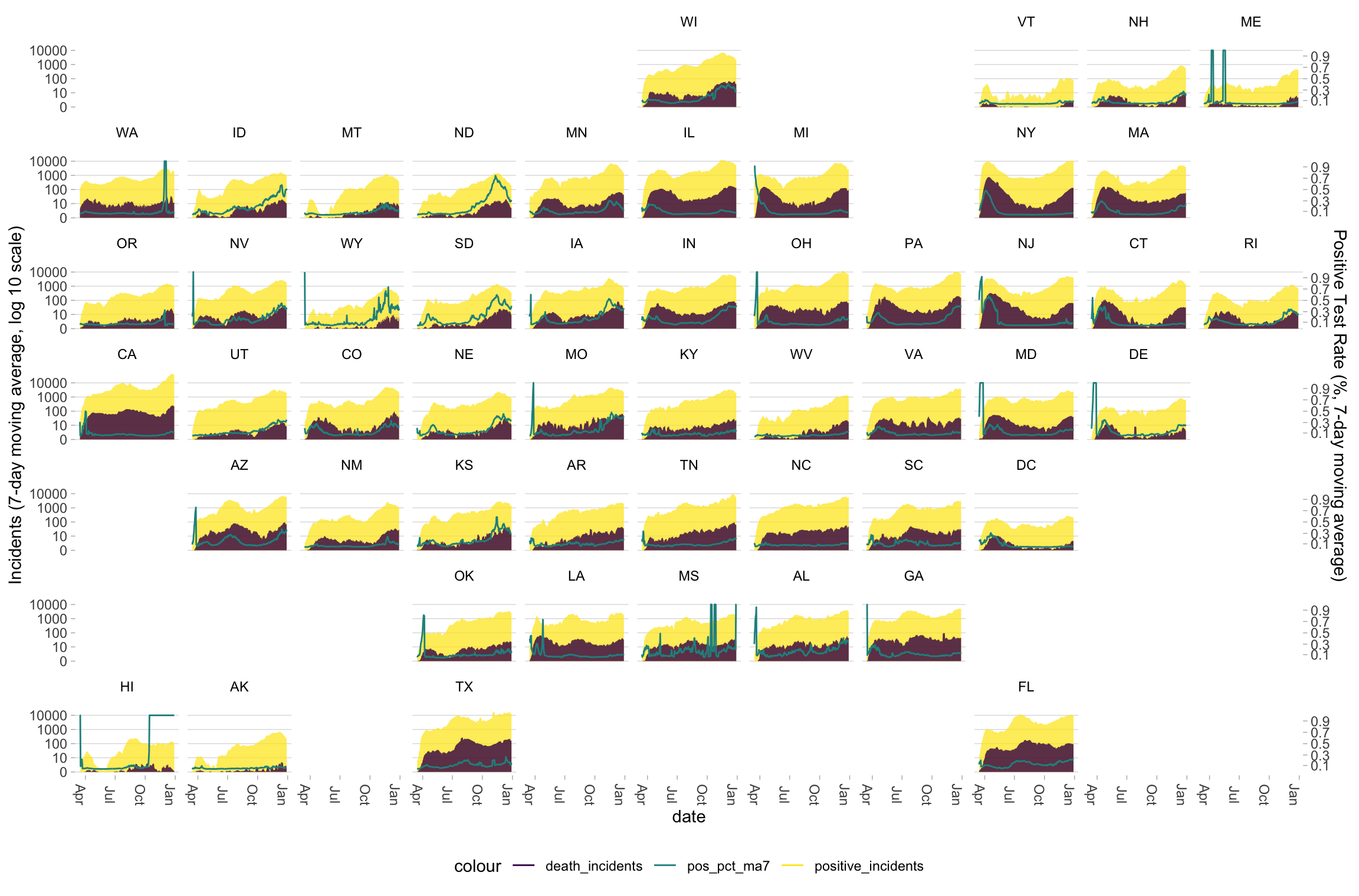
6.4 Plotting multiple geographic units (example: all Washington state counties)
We can do something similar at a county level within states using JHU data, which doesn’t include testing information. At the county level, the data are even noisier.
g_wa <- iusa %>%
  filter(state == "Washington") %>%
  mutate(code_fips = substr(fips, 3, 5)) %>%
  ggplot(aes(x = date))

g_wa +
  geom_area(aes(y = ma7, fill = subset), alpha = .75) +
  scale_y_continuous(trans = scales::pseudo_log_trans(base = 10),
                   name = "Incidents (7-day moving average, log 10 scale)", breaks = c(0, 10, 100, 1000)) +
  scale_color_viridis_d(direction = -1) +
  scale_fill_viridis_d(direction = -1) +
  guides(alpha = "none") +
  facet_geo(~ county, grid = "us_wa_counties_grid1", label = "name", move_axes = FALSE) +
  theme_light2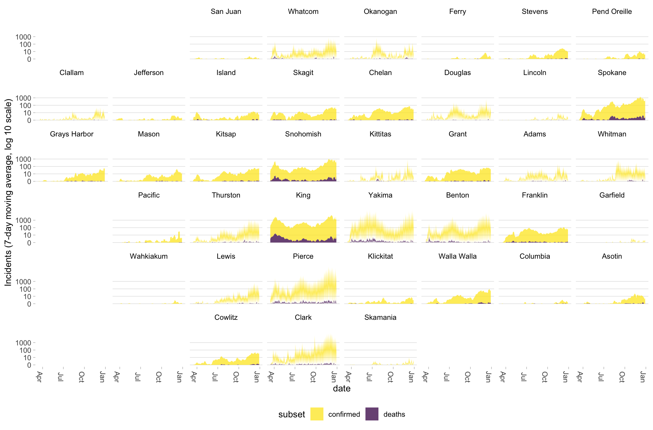
6.5 Extending geographic facets to other regions
Many additional grids are built-in to {geofacet}.
##   [1] "us_state_grid1"
##   [2] "us_state_grid2"
##   [3] "eu_grid1"
##   [4] "aus_grid1"
##   [5] "sa_prov_grid1"
##   [6] "gb_london_boroughs_grid"
##   [7] "nhs_scot_grid"
##   [8] "india_grid1"
##   [9] "india_grid2"
##  [10] "argentina_grid1"
##  [11] "br_states_grid1"
##  [12] "sea_grid1"
##  [13] "mys_grid1"
##  [14] "fr_regions_grid1"
##  [15] "de_states_grid1"
##  [16] "us_or_counties_grid1"
##  [17] "us_wa_counties_grid1"
##  [18] "us_in_counties_grid1"
##  [19] "us_in_central_counties_grid1"
##  [20] "se_counties_grid1"
##  [21] "sf_bay_area_counties_grid1"
##  [22] "ua_region_grid1"
##  [23] "mx_state_grid1"
##  [24] "mx_state_grid2"
##  [25] "scotland_local_authority_grid1"
##  [26] "us_state_without_DC_grid1"
##  [27] "italy_grid1"
##  [28] "italy_grid2"
##  [29] "be_province_grid1"
##  [30] "us_state_grid3"
##  [31] "jp_prefs_grid1"
##  [32] "ng_state_grid1"
##  [33] "bd_upazila_grid1"
##  [34] "spain_prov_grid1"
##  [35] "ch_cantons_grid1"
##  [36] "ch_cantons_grid2"
##  [37] "china_prov_grid1"
##  [38] "world_86countries_grid"
##  [39] "se_counties_grid2"
##  [40] "uk_regions1"
##  [41] "us_state_contiguous_grid1"
##  [42] "sk_province_grid1"
##  [43] "ch_aargau_districts_grid1"
##  [44] "jo_gov_grid1"
##  [45] "spain_ccaa_grid1"
##  [46] "spain_prov_grid2"
##  [47] "world_countries_grid1"
##  [48] "br_states_grid2"
##  [49] "china_city_grid1"
##  [50] "kr_seoul_district_grid1"
##  [51] "nz_regions_grid1"
##  [52] "sl_regions_grid1"
##  [53] "us_census_div_grid1"
##  [54] "ar_tucuman_province_grid1"
##  [55] "us_nh_counties_grid1"
##  [56] "china_prov_grid2"
##  [57] "pl_voivodeships_grid1"
##  [58] "us_ia_counties_grid1"
##  [59] "us_id_counties_grid1"
##  [60] "ar_cordoba_dep_grid1"
##  [61] "us_fl_counties_grid1"
##  [62] "ar_buenosaires_communes_grid1"
##  [63] "nz_regions_grid2"
##  [64] "oecd_grid1"
##  [65] "ec_prov_grid1"
##  [66] "nl_prov_grid1"
##  [67] "ca_prov_grid1"
##  [68] "us_nc_counties_grid1"
##  [69] "mx_ciudad_prov_grid1"
##  [70] "bg_prov_grid1"
##  [71] "us_hhs_regions_grid1"
##  [72] "tw_counties_grid1"
##  [73] "tw_counties_grid2"
##  [74] "af_prov_grid1"
##  [75] "us_mi_counties_grid1"
##  [76] "pe_prov_grid1"
##  [77] "sa_prov_grid2"
##  [78] "mx_state_grid3"
##  [79] "cn_bj_districts_grid1"
##  [80] "us_va_counties_grid1"
##  [81] "us_mo_counties_grid1"
##  [82] "cl_santiago_prov_grid1"
##  [83] "us_tx_capcog_counties_grid1"
##  [84] "sg_planning_area_grid1"
##  [85] "in_state_ut_grid1"
##  [86] "cn_fujian_prov_grid1"
##  [87] "ca_quebec_electoral_districts_grid1"
##  [88] "nl_prov_grid2"
##  [89] "cn_bj_districts_grid2"
##  [90] "ar_santiago_del_estero_prov_grid1"
##  [91] "ar_formosa_prov_grid1"
##  [92] "ar_chaco_prov_grid1"
##  [93] "ar_catamarca_prov_grid1"
##  [94] "ar_jujuy_prov_grid1"
##  [95] "ar_neuquen_prov_grid1"
##  [96] "ar_san_luis_prov_grid1"
##  [97] "ar_san_juan_prov_grid1"
##  [98] "ar_santa_fe_prov_grid1"
##  [99] "ar_la_rioja_prov_grid1"
## [100] "ar_mendoza_prov_grid1"
## [101] "ar_salta_prov_grid1"
## [102] "ar_rio_negro_prov_grid1"
## [103] "uy_departamentos_grid1"
## [104] "ar_buenos_aires_prov_electoral_dist_grid1"
## [105] "europe_countries_grid1"
## [106] "argentina_grid2"
## [107] "us_state_without_DC_grid2"
## [108] "jp_prefs_grid2"
## [109] "na_regions_grid1"
## [110] "mm_state_grid1"
## [111] "us_state_with_DC_PR_grid1"
## [112] "fr_departements_grid1"
## [113] "ar_salta_prov_grid2"
## [114] "ie_counties_grid1"
## [115] "sg_regions_grid1"
## [116] "us_ny_counties_grid1"
## [117] "ru_federal_subjects_grid1"
## [118] "us_ca_counties_grid1"
## [119] "lk_districts_grid1"
## [120] "us_state_without_DC_grid3"
## [121] "co_cali_subdivisions_grid1"
## [122] "us_in_northern_counties_grid1"
## [123] "italy_grid3"
## [124] "us_state_with_DC_PR_grid2"
## [125] "us_state_grid7"
## [126] "sg_planning_area_grid2"
## [127] "ch_cantons_fl_grid1"
## [128] "europe_countries_grid2"
## [129] "us_states_territories_grid1"
## [130] "us_tn_counties_grid1"
## [131] "us_il_chicago_community_areas_grid1"
## [132] "us_state_with_DC_PR_grid3"
## [133] "in_state_ut_grid2"
## [134] "at_states_grid1"
## [135] "us_pa_counties_grid1"
## [136] "us_oh_counties_grid1"
## [137] "fr_departements_grid2"
## [138] "us_wi_counties_grid1"
## [139] "africa_countries_grid1"
## [140] "no_counties_grid1"
## [141] "tr_provinces_grid1"
For states or other regions that aren’t yet included in {geofacet}’s grids, you can construct one using the Geo Grid Designer. For more information, see the geofacet page on CRAN.