Estimate R(t) for all locales in a case-tracking dataset

This function can estimate R(t) curves for all locations in a case-tracking dataset and return a stacked data.frame with the location details included. It is a convenience function for getting R(t) over a large dataset. Right now, nothing is done in "parallel", so this function is not going to be much (or any) faster than running on each location in a case-tracking dataset independently and then combining.

bulk_estimate_Rt(
  df,
  grouping_columns = setdiff(colnames(df), c(cases_column, date_column)),
  cases_column = "count",
  date_column = "date",
  ...
)

Arguments

df

a data.frame containing at least a date column and a cases column, describing the cumulative cases at each date. The data.frame may contain additional columns that can be used to "group" the dates and cases to produce a set of R(t) curves.

grouping_columns

character() vector specifying the grouping columns that will break df into chunks for estimation (i.e., location, etc.). The default is normally correct and includes all columns except for date_column and case_column.

cases_column

character(1) the column in df that includes the case counts of interest.

date_column

character(1) the column in df that includes the date information about when cases reported.

...

passed on to estimate_Rt

Value

A "stacked" data.frame with the outputs from the R(t) estimation process and associated location information. The actual columns returned for the R(t) estimate will depend on the estimation_family parameter as well as other parameters specific to each method.

See also

Other analysis: estimate_Rt()

Other case-tracking: align_to_baseline(), beoutbreakprepared_data(), combined_us_cases_data(), coronadatascraper_data(), covidtracker_data(), ecdc_data(), estimate_Rt(), jhu_data(), nytimes_county_data(), owid_data(), plot_epicurve(), test_and_trace_data(), usa_facts_data(), who_cases()

Author

Sean Davis seandavi@gmail.com

Examples

library(dplyr)
nyt = nytimes_state_data() %>% 
    dplyr::filter(subset=='confirmed') %>%
    dplyr::arrange(state,date)
head(nyt)
#> # A tibble: 6 × 5
#>   date       state   fips  count subset   
#>   <date>     <chr>   <chr> <dbl> <chr>    
#> 1 2020-03-13 Alabama 00001     6 confirmed
#> 2 2020-03-14 Alabama 00001    12 confirmed
#> 3 2020-03-15 Alabama 00001    23 confirmed
#> 4 2020-03-16 Alabama 00001    29 confirmed
#> 5 2020-03-17 Alabama 00001    39 confirmed
#> 6 2020-03-18 Alabama 00001    51 confirmed

# this may produce warnings, but the processing
# will still be correct....
res = bulk_estimate_Rt(head(nyt,500), 
    estimation_family='epiestim',method = 'parametric_si',
    config = list(mean_si=3.96, std_si=4.75))
#> Warning: All elements of `...` must be named.
#> Did you want `data = -c(grouping_columns)`?
head(res)
#> # A tibble: 6 × 17
#>   state  fips  subset data     t_start t_end `Mean(R)` `Std(R)` `Quantile.0.02…`
#>   <chr>  <chr> <chr>  <list>     <dbl> <dbl>     <dbl>    <dbl>            <dbl>
#> 1 Alaba… 00001 confi… <tibble>       2     8      2.44    0.242             1.98
#> 2 Alaba… 00001 confi… <tibble>       3     9      2.00    0.183             1.66
#> 3 Alaba… 00001 confi… <tibble>       4    10      1.75    0.150             1.46
#> 4 Alaba… 00001 confi… <tibble>       5    11      1.81    0.139             1.54
#> 5 Alaba… 00001 confi… <tibble>       6    12      1.78    0.125             1.55
#> 6 Alaba… 00001 confi… <tibble>       7    13      2.39    0.130             2.14
#> # … with 8 more variables: `Quantile.0.05(R)` <dbl>, `Quantile.0.25(R)` <dbl>,
#> #   `Median(R)` <dbl>, `Quantile.0.75(R)` <dbl>, `Quantile.0.95(R)` <dbl>,
#> #   `Quantile.0.975(R)` <dbl>, date_start <date>, date_end <date>
colnames(res)
#>  [1] "state"             "fips"              "subset"           
#>  [4] "data"              "t_start"           "t_end"            
#>  [7] "Mean(R)"           "Std(R)"            "Quantile.0.025(R)"
#> [10] "Quantile.0.05(R)"  "Quantile.0.25(R)"  "Median(R)"        
#> [13] "Quantile.0.75(R)"  "Quantile.0.95(R)"  "Quantile.0.975(R)"
#> [16] "date_start"        "date_end"         

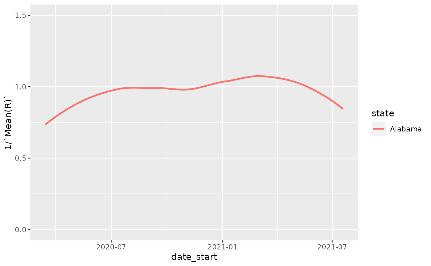
library(ggplot2)
ggplot(res, aes(x=date_start,y=1/`Mean(R)`,color=state)) + 
    geom_smooth(se=FALSE) + ylim(c(0,1.5))
#> `geom_smooth()` using method = 'loess' and formula 'y ~ x'
#> Warning: Removed 16 rows containing non-finite values (stat_smooth).