mtcars data

We are going to use the mtcars dataset, included with R, to experiment with ggplot2.

data(mtcars)

• Exercise: Explore the mtcars dataset using View, summary, dim, class, etc.

We can also take a quick look at the relationships between the variables using the pairs plotting function.

pairs(mtcars)

That is a useful view of the data. We want to use ggplot2 to make an informative plot, so let’s approach this in a piecewise fashion. We first need to decide what type of plot to produce and what our basic variables will be. In this case, we have a number of choices.

ggplot(mtcars,aes(x=disp,y=hp))

First, a little explanation is necessary. The ggplot function takes as its first argument a data.frame. The second argument is the “aesthetic”, aes. The x and y take column names from the mtcars data.frame and will form the basis of our scatter plot.

But why did we get that “Error: No layers in plot”? Remember that ggplot2 is a “grammar of graphics”. We supplied a subject, but no verb (called a layer by ggplot2). So, to generate a plot, we need to supply a verb. There are many possibilities. Each “verb” or layer typically starts with “geom” and then a descriptor. An example is necessary.

ggplot(mtcars,aes(x=disp,y=hp)) + geom_point()

We finally produced a plot. The power of ggplot2, though, is the ability to make very rich plots by adding “grammar” to the “plot sentence”. We have a number of other variables in our mtcars data.frame. How can we add another value to a two-dimensional plot?

ggplot(mtcars,aes(x=disp,y=hp,color=cyl)) + geom_point()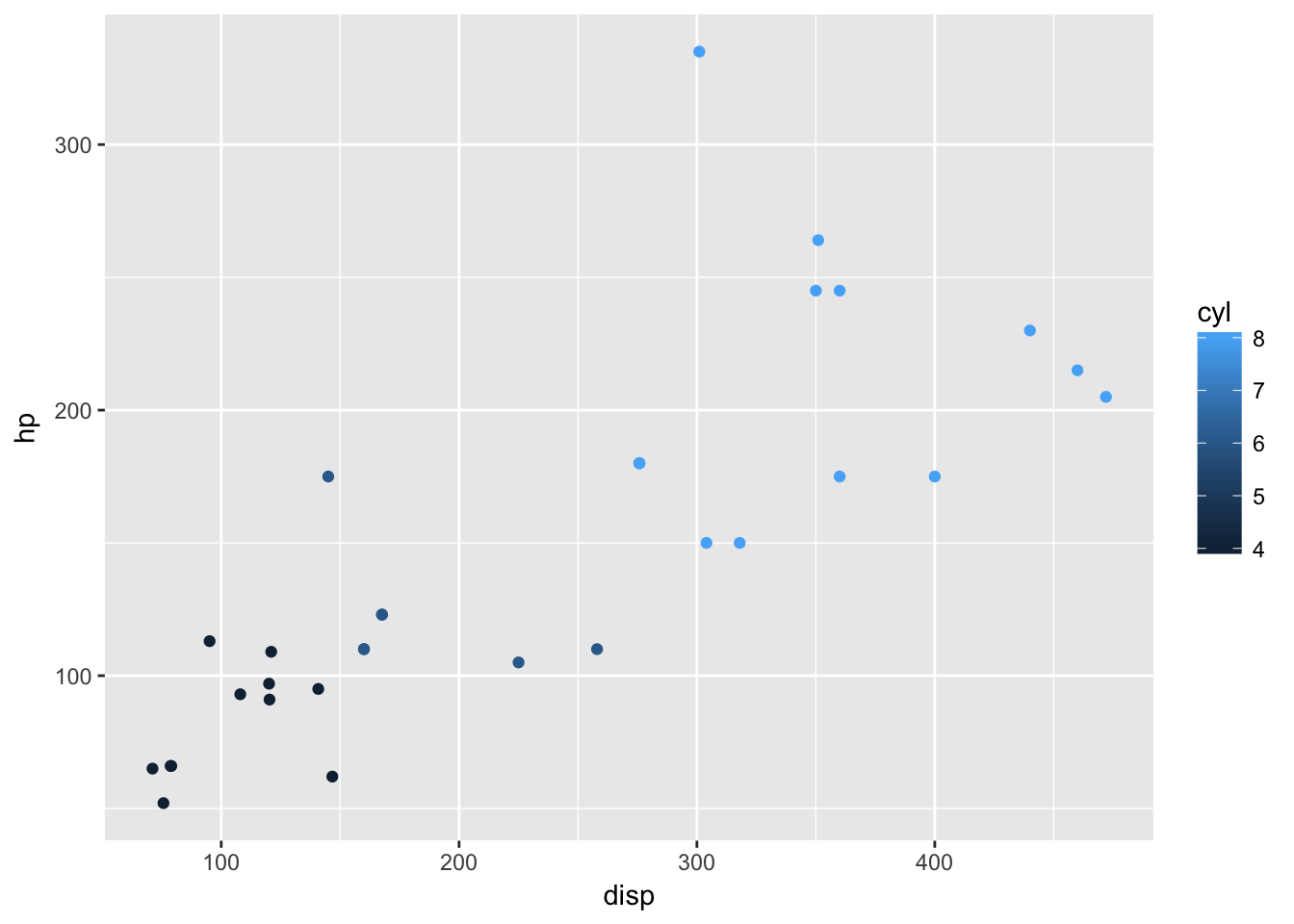

The color of the points is a based on the numeric variable wt, the weight of the car. Can we do more? We can change the size of the points, also.

ggplot(mtcars,aes(x=disp,y=hp,color=wt,size=mpg)) + geom_point()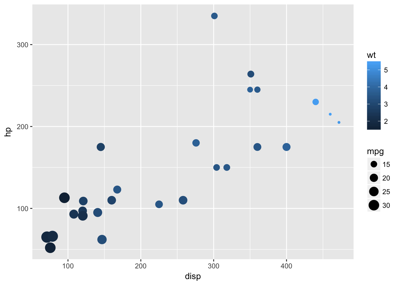

So, on our 2D plot, we are now plotting four variables. Can we do more? We can manipulate the shape of the points in addition to the color and the size.

ggplot(mtcars,aes(x=disp,y=hp)) + geom_point(aes(size=mpg,color=wt,shape=cyl))

Why did we get that error? Ggplot2 is trying to be helpful by telling us that a “continuous varialbe cannot be mapped to ‘shape’”. Well, in our mtcars data.frame, we can look at cyl in detail.

class(mtcars$cyl)

## [1] "numeric"

summary(mtcars$cyl)

##    Min. 1st Qu.  Median    Mean 3rd Qu.    Max. 
##   4.000   4.000   6.000   6.188   8.000   8.000

table(mtcars$cyl)

## 
##  4  6  8 
## 11  7 14

The cyl variable is “kinda” continuous in that it is numeric, but it could also be thought of as a “category” of engines. R has a specific data type for “category” data, called a factor. We can easily convert the cyl column to a factor like so:

mtcars$cyl = as.factor(mtcars$cyl)

Now, we can go ahead with our previous approach to make a 2-dimensional plot that displays the relationships between five variables.

ggplot(mtcars,aes(x=disp,y=hp)) + geom_point(aes(size=mpg,color=wt,shape=cyl))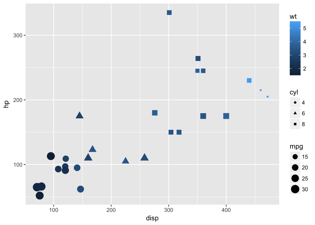

NYC Flight data

I leave this section open-ended for you to explore further options with the ggplot2 package. The data represent the on-time data for all flights that departed New York City in 2013.

library(nycflights13)
head(flights)

## # A tibble: 6 × 19
##    year month   day dep_time sched_dep_time dep_delay arr_time
##   <int> <int> <int>    <int>          <int>     <dbl>    <int>
## 1  2013     1     1      517            515         2      830
## 2  2013     1     1      533            529         4      850
## 3  2013     1     1      542            540         2      923
## 4  2013     1     1      544            545        -1     1004
## 5  2013     1     1      554            600        -6      812
## 6  2013     1     1      554            558        -4      740
## # ... with 12 more variables: sched_arr_time <int>, arr_delay <dbl>,
## #   carrier <chr>, flight <int>, tailnum <chr>, origin <chr>, dest <chr>,
## #   air_time <dbl>, distance <dbl>, hour <dbl>, minute <dbl>,
## #   time_hour <dttm>

Feel free to explore. Consider using other “geoms” during your exploration.