Wednesday, December 07, 2016
Introduction
What is R?
- A software package
- A programming language
- A toolkit for developing statistical and analytical tools
- An extensive library of statistical and mathematical software and algorithms
- A scripting language
- …
Why R?
- R is cross-platform and runs on Windows, Mac, and Linux (as well as more obscure systems).
- R provides a vast number of useful statistical tools, many of which have been painstakingly tested.
- R produces publication-quality graphics in a variety of formats.
- R plays well with FORTRAN, C, and scripts in many languages.
- R scales, making it useful for small and large projects. It is NOT Excel.
- R eschews the GUI.
I can develop code for analysis on my Mac laptop. I can then install the same code on our massive computer cluster and run it in parallel on 1000 samples, monitor the process, and then update a database with R when complete.
Why not R?
- R cannot do everything.
- R is not always the ``best'' tool for the job.
- R will \textit{not hold your hand.
- The documentation can be opaque.
- R can drive you crazy (on a good day) or age you prematurely (on a bad one).
- Finding the right package to do the job you want to do can be challenging; worse, some contributed packages are unreliable.
- R eschews the GUI.
R License and the Open Source Ideal
- R is free!
- Distributed under GNU license
- You may download the source code.
- You may modify the source code to your heart's content.
- You may distribute the modified source code and even charge money for it,
- but you must distribute the modified source code under the original GNU license
Take-home Message
This license means that R will always be available, will always be open source, and can grow organically without constraint.
Getting started
Installation
The first step is to install R. You can download and install R from the Comprehensive R Archive Network (CRAN). It is relatively straightforward, but if you need further help you can try the following resources:
Installing RStudio
The next step is to install RStudio, a program for viewing and running R scripts. Technically you can run all the code shown here without installing RStudio, but we highly recommend this integrated development environment (IDE).
R on your own
Try out the swirl tutorial, which teaches you R programming and data science interactively, at your own pace and in the R console. Once you have R installed, you can install swirl and run it the following way:
install.packages("swirl")
library(swirl)
swirl()
Quick R references
There are also many open and free resources and reference guides for R. Two examples are:
R from zero
Follow along
- In RStudio, copy and paste the following:
download.file('https://raw.githubusercontent.com/seandavi/hour_of_code/master/HourOfCode.Rmd',
              destfile='HourOfCode.Rmd')
- In the file pane, you can choose the
HourOfCode.Rmdfile and it will open in the RStudio text pane.
Interacting with R
Expression
1 + pi + sin(3.7)
## [1] 3.611757
Assignment
x = 1
y <- 2
3 -> z
Interacting with R
- The
<-,->and=are all assignment operators.
x = 1
y <- 2
3 -> z
- If a line is not a complete R command, R will continue the next line with a
+.
1 + pi +
    sin(3.7)
Getting help
R has extensive help functionality built in.
help('print')
help(print)
?print
?data.frame
?`+`
help.search('microarray')
RSiteSearch('microarray')
- For any new function that you see, type
help(newfunction).
First steps in R
Paths and the Working Directory
When you are working in R it is useful to know your working directory. This is the directory or folder in which R will save or look for files by default. You can see your working directory by typing:
getwd()
Loading data into R
R can read files of many different types and from many different sources.
Directly from the web
dir <- "https://raw.githubusercontent.com/genomicsclass/dagdata/master/inst/extdata/"
url <- paste0(dir, "femaleMiceWeights.csv")
dat <- read.csv(url)
Download first
library(downloader) ##use install.packages to install
dir <- "https://raw.githubusercontent.com/genomicsclass/dagdata/master/inst/extdata/"
filename <- "femaleMiceWeights.csv"
url <- paste0(dir, filename)
if (!file.exists(filename)) download(url, destfile=filename)
Working with data
head(dat)
tail(dat)
summary(dat)
dim(dat)
Working with data
head(dat)
##   Diet Bodyweight
## 1 chow      21.51
## 2 chow      28.14
## 3 chow      24.04
## 4 chow      23.45
## 5 chow      23.68
## 6 chow      19.79
Working with data
tail(dat)
##    Diet Bodyweight
## 19   hf      29.58
## 20   hf      30.92
## 21   hf      34.02
## 22   hf      21.90
## 23   hf      31.53
## 24   hf      20.73
Working with data
summary(dat)
##    Diet      Bodyweight
##  chow:12   Min.   :19.79
##  hf  :12   1st Qu.:22.36
##            Median :25.16
##            Mean   :25.32
##            3rd Qu.:28.14
##            Max.   :34.02
Working with data
dim(dat)
## [1] 24 2
dplyr
dplyr filter
library(dplyr)
chow <- filter(dat, Diet=="chow") #keep only the ones with chow diet
head(chow)
##   Diet Bodyweight
## 1 chow      21.51
## 2 chow      28.14
## 3 chow      24.04
## 4 chow      23.45
## 5 chow      23.68
## 6 chow      19.79
dplyr select
chowVals <- select(chow,Bodyweight)
head(chowVals)
##   Bodyweight
## 1      21.51
## 2      28.14
## 3      24.04
## 4      23.45
## 5      23.68
## 6      19.79
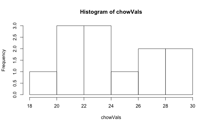
Piping
chowVals <- filter(dat, Diet=="chow") %>% select(Bodyweight) %>% unlist
hist(chowVals)
Plotting with ggplot2
ggplot2 package
The ggplot2 package is a relatively novel approach to generating highly informative publication-quality graphics. The "gg" stands for "Grammar of Graphics". In short, instead of thinking about a single function that produces a plot, ggplot2 uses a "grammar" approach, akin to building more and more complex sentences to layer on more information or nuance.
Data Model
The ggplot2 package assumes that data are in the form of a data.frame. In some cases, the data will need to be manipulated into a form that matches assumptions that ggplot2 uses. In particular, if one has a matrix of numbers associated with different subjects (samples, people, etc.), the data will usually need to be transformed into a "long" data frame.
Getting started
To use the ggplot2 package, it must be installed and loaded. Assuming that installation has been done already, we can load the package directly:
library(ggplot2)
Playing with ggplot2
mtcars data
We are going to use the mtcars dataset, included with R, to experiment with ggplot2.
data(mtcars)
- Exercise: Explore the
mtcarsdataset usingView,summary,dim,class, etc.
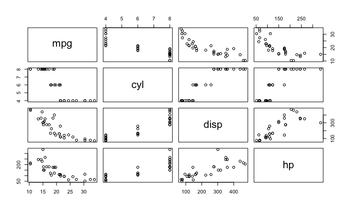
Pairs plot
We can also take a quick look at the relationships between the variables using the pairs plotting function.
pairs(mtcars[,1:4])
Go to the vignette
download.file('https://raw.githubusercontent.com/seandavi/hour_of_code/master/ggplot2.Rmd',
              destfile='ggplot2.Rmd')
Reproducibility
Literate programming
- See the code for these slides
- R markdown
sessionInfo
sessionInfo()
## R Under development (unstable) (2016-10-26 r71594)
## Platform: x86_64-apple-darwin13.4.0 (64-bit)
## Running under: macOS Sierra 10.12.1
##
## locale:
## [1] en_US.UTF-8/en_US.UTF-8/en_US.UTF-8/C/en_US.UTF-8/en_US.UTF-8
##
## attached base packages:
## [1] stats     graphics  grDevices utils     datasets  base
##
## other attached packages:
## [1] ggplot2_2.2.0 dplyr_0.5.0   knitr_1.15.1
##
## loaded via a namespace (and not attached):
##  [1] Rcpp_0.12.8.2      digest_0.6.10      rprojroot_1.1
##  [4] assertthat_0.1     plyr_1.8.4         grid_3.4.0
##  [7] R6_2.2.0           gtable_0.2.0       DBI_0.5-1
## [10] backports_1.0.4    magrittr_1.5       scales_0.4.1
## [13] evaluate_0.10      stringi_1.1.2      lazyeval_0.2.0
## [16] rmarkdown_1.2.9000 tools_3.4.0        stringr_1.1.0
## [19] munsell_0.4.3      yaml_2.1.14        colorspace_1.3-1
## [22] htmltools_0.3.5    methods_3.4.0      tibble_1.2