Multivariate survival analysis
Application to TARGET Osteosarcoma metastatic and single sample GSEA results
Sean Davis1
2020-05-20
Source:vignettes/multivariate_survival.Rmd
multivariate_survival.RmdAbstract
The goal of this workflow is to showcase how to use Cox regression in R to analyze a combination of continuous and categorical predictors of survival. The dataset is from the TARGET osteosarcoma project. The continuous variable(s) are derived elsewhere, but are the results of applying single sample Gene Set Enrichment Analysis (GSEA) to a group of “interesting” biological genes.Learning goals and objectives
- Know that Kaplan-Meier is a univariate statistical approach.
- Know that Kaplan-Meier is applicable only to categorical variables.
- Know that Cox regression can be applied to univariate or multivariate data with both categorical or continuous predictors.
- Understand how to use
anova()to determine the statistical significance of predictors. - Be able to apply
anova()to determine if an additional predictor is helpful to predicting survival. - Be able to identify and interpret the Hazard Ratios from a Cox regression model.
Setup
We need a few R packages to get going. If these are not installed, install them first. To install the TargetOsteoAnalysis package requires a little extra work:
BiocManager::install('seandavi/TargetOsteoAnalysis')
The dataset
The following code loads data from the TargetOsteoAnalysis package and then manipulates it to be a bit simpler for the workflow below.
ssgsea_survival = read.delim(
  system.file('extdata/All_ssGSEA_CTA4surv.txt.gz',
              package='TargetOsteoAnalysis'),
  sep="\t") %>%
  dplyr::mutate(status=Vital.Status=='Dead',
                time = Overall.Survival.Time.in.Days,
                gender = stringr::str_trim(Gender),
                metastatic = Disease.at.diagnosis) %>%
  dplyr::select(status,time,metastatic,CTA_chrX,CTA_all,gender)
Introduction
The Cox proportional-hazards model (Cox 1972) is semi-parametric regression model commonly used for investigating the association between the survival time of patients and one or more predictor variables. Kaplan-Meier curves and logrank tests - are examples of univariate analysis approaches. They can be applied in the setting of one factor under investigation, but ignore the impact of any others. Additionally, Kaplan-Meier curves and logrank tests are useful only when the predictor variable is categorical (e.g.: treatment A vs treatment B; males vs females). They don’t work easily for quantitative predictors such as gene expression, weight, or age without binning the variable first to create categories
Cox proportional hazards regression analysis works for both quantitative predictor variables and for categorical variables. Furthermore, the Cox regression model extends survival analysis methods to assess simultaneously the effect of several risk factors on survival time; ie., Cox regression can be multivariate.
Kaplan-Meier/LogRank test vs Cox Regression
surv_met_fit= survfit(
  survival::Surv(time,status) ~ metastatic,
  data=ssgsea_survival)
survminer::ggsurvplot(surv_met_fit, risk.table = TRUE)
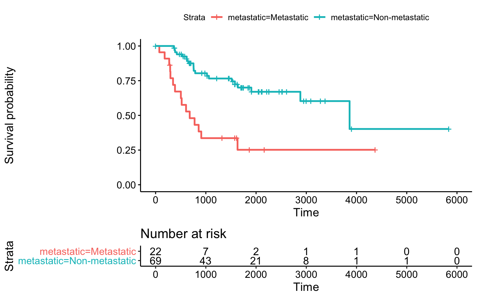
Simple Kaplan-Meier survival plot with metastatic status at diagnosis.
To perform the actual logrank testing, we apply the survdiff() function. This function tests if there is a difference between two or more survival curves using the G-rho family of tests (Harrington and Fleming 1982).
surv_km  = survdiff(
  survival::Surv(time,status) ~ metastatic,
  data=ssgsea_survival)
surv_km
#> Call:
#> survdiff(formula = survival::Surv(time, status) ~ metastatic,
#>     data = ssgsea_survival)
#>
#>                            N Observed Expected (O-E)^2/E (O-E)^2/V
#> metastatic=Metastatic     22       15     5.96     13.74      16.7
#> metastatic=Non-metastatic 69       20    29.04      2.82      16.7
#>
#>  Chisq= 16.7  on 1 degrees of freedom, p= 4e-05
So, the p-value for this test, also known as the log-rank or Mantel-Haenszel test, is 4.304057810^{-5}.
Regression approaches allow us to treat categorical and continuous variables in a common statistical framework. Here, we apply the coxph() method to perform Cox regression with the categorical variable, metastatic, as the predictor. Note that the exact same model formula is used here, but the testing procedure is different.
We can look at the Cox regression results using the summary() method:
summary(surv_met)
#> Call:
#> survival::coxph(formula = survival::Surv(time, status) ~ metastatic,
#>     data = ssgsea_survival)
#>
#>   n= 91, number of events= 35
#>
#>                             coef exp(coef) se(coef)      z Pr(>|z|)
#> metastaticNon-metastatic -1.3177    0.2677   0.3451 -3.818 0.000134 ***
#> ---
#> Signif. codes:  0 '***' 0.001 '**' 0.01 '*' 0.05 '.' 0.1 ' ' 1
#>
#>                          exp(coef) exp(-coef) lower .95 upper .95
#> metastaticNon-metastatic    0.2677      3.735    0.1361    0.5266
#>
#> Concordance= 0.664  (se = 0.041 )
#> Likelihood ratio test= 12.97  on 1 df,   p=3e-04
#> Wald test            = 14.58  on 1 df,   p=1e-04
#> Score (logrank) test = 16.73  on 1 df,   p=4e-05
Digging through this result can be a bit challenging. Let’s start at the bottom. The three results, Likelihood ratio test, Wald test, and Score (logrank) test with p=... are omnibus tests that report the results of three different testing procedures for the entire model. In particular, note that the p-value for the Score (logrank) test is identical to the p-value of the logrank test from the survdiff results above.
The next block of rows (exp(coef), exp(-coef), lower .95, upper .95) report the hazard ratios. The exp(coef) is the Hazard Ratio associated with metastaticNon-metastatic condition. This may seem a strange way to report things, but the assumption is that the “baseline” is the metasticMetastatic condition; thus, the hazard ratio reported here, 0.2677, suggests that “Non-metastatic” is protective. The “lower” and “upper” confidence intervals (lower .95, upper .95) do not intersect a hazard ratio of 1, so we would expect the effect to be significant.
Moving up to the next block of rows, we can find the p-value for the specific variable (Pr(>|z|)). The p-value reported here is identical to the p-value for the Wald Test, 1.343327410^{-4}.
Looking at CTA genes
We can apply the same Cox regression procedure for the continuous variable, CTA_all, for example.
surv_cta_all = survival::coxph(
  survival::Surv(time,status) ~ CTA_chrX,
  data=ssgsea_survival)
summary(surv_cta_all)
#> Call:
#> survival::coxph(formula = survival::Surv(time, status) ~ CTA_chrX,
#>     data = ssgsea_survival)
#>
#>   n= 91, number of events= 35
#>
#>                coef  exp(coef)   se(coef)      z Pr(>|z|)
#> CTA_chrX -0.0003237  0.9996764  0.0001206 -2.683  0.00729 **
#> ---
#> Signif. codes:  0 '***' 0.001 '**' 0.01 '*' 0.05 '.' 0.1 ' ' 1
#>
#>          exp(coef) exp(-coef) lower .95 upper .95
#> CTA_chrX    0.9997          1    0.9994    0.9999
#>
#> Concordance= 0.679  (se = 0.05 )
#> Likelihood ratio test= 9.9  on 1 df,   p=0.002
#> Wald test            = 7.2  on 1 df,   p=0.007
#> Score (logrank) test = 8.01  on 1 df,   p=0.005
Again, looking at the omnibus tests, all are significant for the entire model. The Hazard Ratio estimate is 0.9997 which is interpreted to mean that higher ssGSEA scores for the CTA genes is protective.
Now, how can we include metastasis and the ssGSEA results in the same model? Programmatically, we can just include a + in the model formula. That looks like:
surv_full = survival::coxph(
  survival::Surv(time,status) ~ metastatic + CTA_all,
  data=ssgsea_survival)
Does adding CTA_all to the model make a significance difference? The way to address the question of whether a model that includes more covariates is “better” than one with fewer is to formally test. In particular, we need to have the model without the CTA_all results and compare it to the same model but with the CTA_all results included.
The model with only metastasis looks like:
We use the anova() method to compare models:
anova(surv_met_only,surv_full)
#> Analysis of Deviance Table
#>  Cox model: response is  survival::Surv(time, status)
#>  Model 1: ~ metastatic
#>  Model 2: ~ metastatic + CTA_all
#>    loglik  Chisq Df P(>|Chi|)
#> 1 -133.51
#> 2 -128.78 9.4759  1  0.002082 **
#> ---
#> Signif. codes:  0 '***' 0.001 '**' 0.01 '*' 0.05 '.' 0.1 ' ' 1
The results are comparing model 1 that includes only metastasis as a covariate vs model 2 that includes both metastasis and CTA_all. The equivalence of the two models is easily “rejected” since the p-value (P(>|Chi|)) is small.
R has a convenient means to examine a single model using anova(). If we have the full model only, for example, calling anova() on that model will return the results of each “submodel” with variables added in the order of the model formula. You’ll note above that I specified metastatic + CTA_all, so the base model will include no covariates, model 1 will include metastatic status, and model 2 will include both covariates.
anova(surv_full)
#> Analysis of Deviance Table
#>  Cox model: response is survival::Surv(time, status)
#> Terms added sequentially (first to last)
#>
#>             loglik   Chisq Df Pr(>|Chi|)
#> NULL       -140.00
#> metastatic -133.51 12.9740  1  0.0003158 ***
#> CTA_all    -128.78  9.4759  1  0.0020819 **
#> ---
#> Signif. codes:  0 '***' 0.001 '**' 0.01 '*' 0.05 '.' 0.1 ' ' 1
We can see that adding metastatic is signficant. Given that metastatic is in the model, adding CTA_all is also significant.
What about CTA_chrX as a covariate?
surv_full_X = survival::coxph(
  survival::Surv(time,status) ~ metastatic + CTA_chrX,
  data=ssgsea_survival)
anova(surv_full_X)
#> Analysis of Deviance Table
#>  Cox model: response is survival::Surv(time, status)
#> Terms added sequentially (first to last)
#>
#>             loglik  Chisq Df Pr(>|Chi|)
#> NULL       -140.00
#> metastatic -133.51 12.974  1  0.0003158 ***
#> CTA_chrX   -128.01 11.003  1  0.0009099 ***
#> ---
#> Signif. codes:  0 '***' 0.001 '**' 0.01 '*' 0.05 '.' 0.1 ' ' 1
So, it looks like CTA_chrX results also add value to the model. How about including everything?
Including both “CTA” result sets looks like:
surv_all = survival::coxph(
  survival::Surv(time,status) ~ metastatic + CTA_chrX + CTA_all,
  data=ssgsea_survival)
anova(surv_all)
#> Analysis of Deviance Table
#>  Cox model: response is survival::Surv(time, status)
#> Terms added sequentially (first to last)
#>
#>             loglik   Chisq Df Pr(>|Chi|)
#> NULL       -140.00
#> metastatic -133.51 12.9740  1  0.0003158 ***
#> CTA_chrX   -128.01 11.0026  1  0.0009099 ***
#> CTA_all    -127.66  0.7079  1  0.4001532
#> ---
#> Signif. codes:  0 '***' 0.001 '**' 0.01 '*' 0.05 '.' 0.1 ' ' 1
And, for completeness, let’s switch the ordering of the CTA sets?
surv_all = survival::coxph(
  survival::Surv(time,status) ~ metastatic + CTA_all + CTA_chrX,
  data=ssgsea_survival)
anova(surv_all)
#> Analysis of Deviance Table
#>  Cox model: response is survival::Surv(time, status)
#> Terms added sequentially (first to last)
#>
#>             loglik   Chisq Df Pr(>|Chi|)
#> NULL       -140.00
#> metastatic -133.51 12.9740  1  0.0003158 ***
#> CTA_all    -128.78  9.4759  1  0.0020819 **
#> CTA_chrX   -127.66  2.2346  1  0.1349540
#> ---
#> Signif. codes:  0 '***' 0.001 '**' 0.01 '*' 0.05 '.' 0.1 ' ' 1
Why does adding another CTA set not help? Looking at the relationship between the two CTA result sets is helpful.
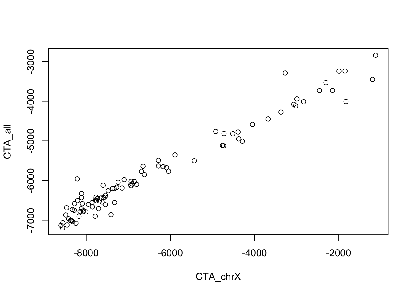
Scatterplot of single sample GSEA scores showing very high correlation between the two
With such high correlation between the two sets (see Figure @ref(fig:ssgsea)), we can understand how including one in the model makes the other irrelevant.
Splitting into two groups first
If we had split the data into “met” and “no-met” groups and then performed the Cox regression, we get the following results:
met_choices = unique(ssgsea_survival$metastatic)
res = lapply(met_choices, function(met) {
  df = ssgsea_survival %>% dplyr::filter(metastatic==met)
  survival::coxph(survival::Surv(time,status) ~ CTA_chrX, data=df)
})
names(res) = met_choices
knitr::kable(
  label = 'metsep',
  dplyr::bind_rows(lapply(res,broom::tidy),.id='met_status'),
  caption = "Cox proportional hazards models to determine the effect of CTA genes on chromosome X (from ssGSEA analysis), applied separately to metastatic and non-metastatic patients. Note that the p-values are not significant when patients are treated separately."
)
| met_status | term | estimate | std.error | statistic | p.value | conf.low | conf.high |
|---|---|---|---|---|---|---|---|
| Non-metastatic | CTA_chrX | -0.0002146 | 0.0001384 | -1.550350 | 0.1210575 | -0.0004858 | 5.67e-05 |
| Metastatic | CTA_chrX | -0.0005132 | 0.0002662 | -1.927684 | 0.0538944 | -0.0010349 | 8.60e-06 |
Checking the p-values for the CTA_chrX covariate in Table @ref(tab:metsep) in each group separately, we see that they are trending in the right direction, but are not significant.
Summary
- Kaplan-Meier and logrank tests have limited application to a single categorical variable
- Cox regression is applicable for both continuous and categorical and can be applied to multiple variables as once.
When working with Cox regression:
References
Cox, D R. 1972. “Regression Models and Life-Tables.” Journal of the Royal Statistical Society. Series B, Statistical Methodology 34 (2):187–202. https://doi.org/10.1111/j.2517-6161.1972.tb00899.x.
Harrington, David P, and Thomas R Fleming. 1982. “A Class of Rank Test Procedures for Censored Survival Data.” Biometrika 69 (3). [Oxford University Press, Biometrika Trust]:553–66. https://doi.org/10.2307/2335991.