Package: HTAN 0.99.1 (source).
This vignette follows one HTAN dataset from a metadata query to a biological result. We pick a small, open spatial transcriptomics section of the colon, confirm where it came from, download it, read it into a SpatialExperiment, wrap it with clinical data in a MultiAssayExperiment, and run a short analysis: quality control, normalisation, clustering and spatial plots. Each step comes with the reason it is done that way.
It assumes you have read the introduction and the data model vignette. The metadata steps run anywhere. The download and every step after it need a free Synapse account and a personal access token in SYNAPSE_AUTH_TOKEN (see the introduction). Where the vignette is built without a token, as on the Bioconductor build machines, that code is shown but not run.
The order matters: the Bioconductor packages attach functions named count(), desc(), slice() and rename() that mask dplyr’s, so dplyr is attached last.
Choosing a dataset
The question
The Vanderbilt atlas (HTA11) studied colorectal precancer and cancer, and a section of colon makes a good first spatial dataset. The colonic mucosa has an obvious architecture (epithelial crypts, the stroma of the lamina propria, immune cells). If the analysis is right, its expression clusters should match recognisable tissue compartments, and agree with what the metadata say the tissue is.
Finding candidate files
10x Visium measures the transcriptome in a grid of 55 µm spots across a tissue section. Level 4 Visium files are processed objects, ready to analyse. These are the open ones, by center and format:
visium <- htan_files(
    assay == "10xVisiumSpatialTranscriptomics-RNA-seq", level == 4,
    access == "open-synapse", con = con)
visium |>
    count(HTAN_Center, extension) |>
    arrange(desc(n)) |>
    collect()
#> # A tibble: 2 × 3
#>   HTAN_Center     extension     n
#>   <chr>           <chr>     <dbl>
#> 1 HTAN WUSTL      .rds        132
#> 2 HTAN Vanderbilt .h5ad        43
Three things guide the choice. The first is format: .h5ad (AnnData) files follow a common layout that anndataR reads reliably, whereas .rds files hold whatever R object the center saved. The second is provenance. We want a file from a single participant, measured on a biospecimen whose tissue type and site are recorded, so the result can be read against them. The third is size, small enough to download in seconds. The biospecimen fields come from the biospecimen table, joined on the assayed biospecimen:
biospecimens <- htan_tbl("biospecimen", con) |>
    select(HTAN_Assayed_Biospecimen_ID = HTAN_Biospecimen_ID,
        Tumor_Tissue_Type, Site_of_Resection_or_Biopsy)
candidates <- visium |>
    filter(extension == ".h5ad", n_participants == 1) |>
    inner_join(biospecimens, by = "HTAN_Assayed_Biospecimen_ID") |>
    filter(Tumor_Tissue_Type != "Not Otherwise Specified",
        Site_of_Resection_or_Biopsy != "Not Reported") |>
    arrange(File_Size) |>
    select(HTAN_Data_File_ID, Filename, File_Size, Tumor_Tissue_Type,
        Site_of_Resection_or_Biopsy) |>
    collect()
nrow(candidates)
#> [1] 25
candidates |>
    transmute(file = basename(Filename), MB = round(File_Size / 1e6),
        Tumor_Tissue_Type, site = Site_of_Resection_or_Biopsy) |>
    head(10)
#> # A tibble: 10 × 4
#>    file                         MB Tumor_Tissue_Type    site
#>    <chr>                     <dbl> <chr>                <chr>
#>  1 8270_AS_1_unfiltered.h5ad    13 Premalignant         Sigmoid colon
#>  2 8270_AS_5_unfiltered.h5ad    13 Atypia - hyperplasia Sigmoid colon
#>  3 8270_AS_2_unfiltered.h5ad    14 Premalignant         Cecum
#>  4 7319_AS_3_unfiltered.h5ad    17 Premalignant         Hepatic flexure of colon
#>  5 7003_AS_1_unfiltered.h5ad    19 Primary              Descending colon
#>  6 8270_AS_3_unfiltered.h5ad    20 Premalignant         Cecum
#>  7 7319_AS_2_unfiltered.h5ad    23 Premalignant         Ascending colon
#>  8 7319_AS_4_unfiltered.h5ad    24 Premalignant         Cecum
#>  9 7003_AS_2_unfiltered.h5ad    24 Primary              Descending colon
#> 10 7794_AS_3_unfiltered.h5ad    32 Primary              Transverse colon
One property that matters is missing from the metadata: the version of AnnData that wrote each file. Files written before AnnData 0.8 (released in 2022) use an older on-disk layout that anndataR does not read. read_htan() reads those with a fallback that keeps the matrices, obs, var and obsm, but drops uns. Every file in this list smaller than 7794_AS_3_unfiltered.h5ad is in the older layout (we checked by opening each one). So we use 7794_AS_3, the smallest file in the current layout, which anndataR reads in full:
visium_id <- "HTA11_99999933430_8422134111"
stopifnot(visium_id %in% candidates$HTAN_Data_File_ID)
file <- htan_files(HTAN_Data_File_ID == visium_id, con = con) |> collect()
glimpse(select(file, HTAN_Data_File_ID, Filename, File_Size, md5,
    entityId, HTAN_Participant_ID, HTAN_Assayed_Biospecimen_ID, access))
#> Rows: 1
#> Columns: 8
#> $ HTAN_Data_File_ID           <chr> "HTA11_99999933430_8422134111"
#> $ Filename                    <chr> "visium_level_4/7794_AS_3_unfiltered.h5ad"
#> $ File_Size                   <dbl> 32435124
#> $ md5                         <chr> "bee3980cc60edb9b1787ad4884daea01"
#> $ entityId                    <chr> "syn51133540"
#> $ HTAN_Participant_ID         <chr> "HTA11_99999933430"
#> $ HTAN_Assayed_Biospecimen_ID <chr> "HTA11_99999933430_84221"
#> $ access                      <chr> "open-synapse"
The entityId is the file’s Synapse ID. access is open-synapse, so you need a token but not a data access request.
What the metadata say about it
The assay table holds the processing details:
workflow <- htan_tbl(
    "10xvisium_spatialtranscriptomics_scRNAseq_level4_metadata", con) |>
    filter(HTAN_Data_File_ID == visium_id) |>
    select(Workflow_Version, Visium_Workflow_Type,
        Visium_Workflow_Parameters_Description, Run_ID, Data_Release) |>
    collect()
glimpse(workflow)
#> Rows: 1
#> Columns: 5
#> $ Workflow_Version                       <chr> "spaceranger-2.0.0"
#> $ Visium_Workflow_Type                   <chr> "Spaceranger 1.3.0"
#> $ Visium_Workflow_Parameters_Description <chr> "transcriptome -- GRCh38-2020-A…
#> $ Run_ID                                 <chr> "7794-AS"
#> $ Data_Release                           <chr> "Release 5.0"
The file was made with Space Ranger against the GRCh38-2020-A reference, with the human whole-transcriptome probe set, so this is the probe-based Visium chemistry. The record disagrees with itself about the Space Ranger version (Workflow_Version is spaceranger-2.0.0, but Visium_Workflow_Type says Spaceranger 1.3.0). These fields were filled in by hand at submission, so read them sceptically. “Unfiltered” in the file name suggests the file holds every spot on the capture area, including those off the tissue; if so, the analysis has to remove them.
Tracing lineage
Before using a processed file, check what it was made from:
lineage <- htan_lineage(visium_id, con = con) |>
    arrange(depth, related_file_id) |>
    collect()
lineage |>
    transmute(depth, Component = sub("10xVisiumSpatialTranscriptomics-",
        "", Component), file = basename(Filename))
#> # A tibble: 8 × 3
#>   depth Component     file
#>   <int> <chr>         <chr>
#> 1    -3 RNA-seqLevel1 7794-AS-3_S1_L005_R1_001.fastq.gz
#> 2    -3 RNA-seqLevel1 7794-AS-3_S1_L005_R2_001.fastq.gz
#> 3    -2 RNA-seqLevel2 7794_AS_3_possorted_genome_bam.bam
#> 4    -1 RNA-seqLevel3 7794_AS_3_barcodes.tsv.gz
#> 5    -1 RNA-seqLevel3 7794_AS_3_features.tsv.gz
#> 6    -1 RNA-seqLevel3 7794_AS_3_matrix.mtx.gz
#> 7    -1 RNA-seqLevel3 7794_AS_3_tissue_positions.csv
#> 8     0 RNA-seqLevel4 7794_AS_3_unfiltered.h5ad
The chain runs from FASTQ (Level 1, controlled) through aligned BAM (Level 2, controlled) and the Space Ranger output (Level 3, open) to this object (Level 4). All were measured on one biospecimen. Here are its record and the participant’s:
biospecimen <- htan_tbl("biospecimen", con) |>
    filter(HTAN_Biospecimen_ID == !!file$HTAN_Assayed_Biospecimen_ID) |>
    select(HTAN_Biospecimen_ID, HTAN_Parent_ID, Acquisition_Method_Type,
        Preservation_Method, Tumor_Tissue_Type, Site_of_Resection_or_Biopsy,
        Histologic_Morphology_Code) |>
    collect()
glimpse(biospecimen)
#> Rows: 1
#> Columns: 7
#> $ HTAN_Biospecimen_ID         <chr> "HTA11_99999933430_84221"
#> $ HTAN_Parent_ID              <chr> "HTA11_99999933430"
#> $ Acquisition_Method_Type     <chr> "Biopsy"
#> $ Preservation_Method         <chr> "unknown"
#> $ Tumor_Tissue_Type           <chr> "Primary"
#> $ Site_of_Resection_or_Biopsy <chr> "Transverse colon"
#> $ Histologic_Morphology_Code  <chr> "0"

htan_tbl("clinical_tier1_demographics", con) |>
    filter(HTAN_Participant_ID == !!file$HTAN_Participant_ID) |>
    select(HTAN_Participant_ID, Gender, Race, Vital_Status) |>
    collect()
#> # A tibble: 1 × 4
#>   HTAN_Participant_ID Gender Race         Vital_Status
#>   <chr>               <chr>  <chr>        <chr>
#> 1 HTA11_99999933430   Male   Not Reported Not Reported

diagnosis <- htan_tbl("clinical_tier1_diagnosis", con) |>
    filter(HTAN_Participant_ID == !!file$HTAN_Participant_ID) |>
    select(Primary_Diagnosis, Morphology, Tissue_or_Organ_of_Origin,
        Tumor_Grade) |>
    collect()
diagnosis
#> # A tibble: 1 × 4
#>   Primary_Diagnosis Morphology   Tissue_or_Organ_of_Origin Tumor_Grade
#>   <chr>             <chr>        <chr>                     <chr>
#> 1 Not Reported      Not Reported Not Reported              Not Reported
The section is a biopsy of the transverse colon, with tissue type “Primary”, HTAN’s term for tissue from a primary tumour (as opposed to premalignant, normal or metastatic tissue). Nothing more specific is recorded: the morphology code is 0 (not reported), and the participant’s primary diagnosis is “Not Reported”. So the metadata do not say whether the lesion is an adenoma or a carcinoma, or of what type, and we have to read the analysis without that. The participant has other data too, which could extend the analysis later:
htan_files(participants = file$HTAN_Participant_ID, con = con) |>
    count(Component, access) |>
    arrange(Component) |>
    collect()
#> # A tibble: 12 × 3
#>    Component                                      access           n
#>    <chr>                                          <chr>        <dbl>
#>  1 10xVisiumSpatialTranscriptomics-AuxiliaryFiles open-synapse     2
#>  2 10xVisiumSpatialTranscriptomics-RNA-seqLevel1  controlled       4
#>  3 10xVisiumSpatialTranscriptomics-RNA-seqLevel2  controlled       2
#>  4 10xVisiumSpatialTranscriptomics-RNA-seqLevel3  open-synapse     8
#>  5 10xVisiumSpatialTranscriptomics-RNA-seqLevel4  open-synapse     2
#>  6 BulkWESLevel1                                  controlled       8
#>  7 BulkWESLevel2                                  controlled       4
#>  8 BulkWESLevel3                                  open-synapse     3
#>  9 ImagingLevel2                                  open-synapse     6
#> 10 ScRNA-seqLevel1                                controlled       2
#> 11 ScRNA-seqLevel2                                controlled       4
#> 12 ScRNA-seqLevel3                                open-synapse    12
Downloading
htan_download() checks the access tier and total size, asks Synapse for a short-lived download URL, fetches the file, and verifies its md5 against the metadata. The file is kept in the package’s download cache (a BiocFileCache under tools::R_user_dir("HTAN", "cache")), so a second call finds the verified copy instead of downloading it again. To get a copy in a directory of your choice as well, pass dest.
dl <- htan_download(file, con = con)
dl
#> # A tibble: 1 × 4
#>   HTAN_Data_File_ID            access       path                          status
#>   <chr>                        <chr>        <chr>                         <chr>
#> 1 HTA11_99999933430_8422134111 open-synapse /github/home/.cache/R/HTAN/d… downl…
Reading into a SpatialExperiment
read_htan() reads .h5ad files with anndataR. When the AnnData object has a spatial embedding (the layout scanpy writes for Visium), the result is a SpatialExperiment with the spot positions as spatialCoords():
spe <- read_htan(dl)
spe
#> class: SpatialExperiment
#> dim: 19338 4992
#> metadata(1): spatial
#> assays(1): X
#> rownames(19338): OR4F5 SAMD11 ... DEPRECATED_ENSG00000284667
#>   DEPRECATED_ENSG00000284704
#> rowData names(10): gene_ids feature_types ...
#>   Median.Normalized.Average.Counts Barcodes.Detected.per.Feature
#> colnames(4992): AAACAACGAATAGTTC-1 AAACAAGTATCTCCCA-1 ...
#>   TTGTTTGTATTACACG-1 TTGTTTGTGTAAATTC-1
#> colData names(14): in_tissue array_row ... kmeans_5_clusters sample_id
#> reducedDimNames(0):
#> mainExpName: NULL
#> altExpNames(0):
#> spatialCoords names(2) : x y
#> imgData names(0):
Level 4 objects differ between centers, so look before you compute. We need to know which assay holds raw counts, whether there are spot coordinates, and which spots are under tissue.
assayNames(spe)
#> [1] "X"
names(colData(spe))
#>  [1] "in_tissue"          "array_row"          "array_col"
#>  [4] "kmeans_7_clusters"  "kmeans_10_clusters" "kmeans_4_clusters"
#>  [7] "kmeans_2_clusters"  "kmeans_6_clusters"  "graphclust"
#> [10] "kmeans_3_clusters"  "kmeans_8_clusters"  "kmeans_9_clusters"
#> [13] "kmeans_5_clusters"  "sample_id"
names(rowData(spe))
#>  [1] "gene_ids"
#>  [2] "feature_types"
#>  [3] "genome"
#>  [4] "n_cells"
#>  [5] "Morans_I"
#>  [6] "Morans_I_p_val"
#>  [7] "Morans_I_adj_p_val"
#>  [8] "Feature.Counts.in.Spots.Under.Tissue"
#>  [9] "Median.Normalized.Average.Counts"
#> [10] "Barcodes.Detected.per.Feature"
head(rownames(spe))
#> [1] "OR4F5"   "SAMD11"  "NOC2L"   "KLHL17"  "PLEKHN1" "PERM1"
is(spe, "SpatialExperiment")
#> [1] TRUE
Marker genes are easier to read as symbols. If the row names are Ensembl IDs, we switch to a symbol column from rowData() (scanpy and Space Ranger name it differently), keeping the names unique. Some probe-set features are named DEPRECATED_ followed by an Ensembl ID. We count them and leave them as they are.
if (mean(grepl("^ENSG", rownames(spe))) > 0.5) {
    symbol_col <- intersect(c("gene_symbols", "gene_name", "feature_name",
        "symbol", "gene_ids"), names(rowData(spe)))[1]
    rownames(spe) <- make.unique(as.character(rowData(spe)[[symbol_col]]))
}
head(rownames(spe))
#> [1] "OR4F5"   "SAMD11"  "NOC2L"   "KLHL17"  "PLEKHN1" "PERM1"
sum(grepl("^DEPRECATED_", rownames(spe)))
#> [1] 332
anndataR maps AnnData’s main matrix X to an assay named X. Whether X holds raw counts or normalised values is up to the center, so we test it. Raw counts are whole numbers.
If this were FALSE, the counts would have to come from a layer of the AnnData object or from the Level 3 Space Ranger matrix listed in the lineage.
If the object has no spatial embedding, the spot positions are in the Level 3 tissue_positions.csv from the lineage table, which can be downloaded and joined by barcode. This chunk does that only when it has to:
if (!is(spe, "SpatialExperiment")) {
    pos_id <- lineage$related_file_id[
        grepl("tissue_positions", lineage$Filename)]
    pos_dl <- htan_download(pos_id, con = con)
    ## Space Ranger 2.0 writes a header row; 1.x did not.
    has_header <- startsWith(readLines(pos_dl$path, n = 1), "barcode")
    pos <- read.csv(pos_dl$path, header = has_header)
    names(pos) <- c("barcode", "in_tissue", "array_row", "array_col",
        "pxl_row", "pxl_col")
    pos <- pos[match(colnames(spe), pos$barcode), ]
    colData(spe)$in_tissue <- pos$in_tissue
    spe <- as(spe, "SpatialExperiment")
    spatialCoords(spe) <- as.matrix(pos[, c("pxl_col", "pxl_row")])
}
dim(spatialCoords(spe))
#> [1] 4992    2
Finally, we keep only spots under tissue. Spots outside it capture ambient RNA and would form a spurious cluster of their own:
Adding clinical context: a MultiAssayExperiment
htan_experiment() builds a MultiAssayExperiment from objects named by their HTAN_Data_File_ID. It looks up each file’s participant in id_provenance, maps every spot to that participant in the sampleMap, and fills colData with the participant’s demographics and diagnosis. Biospecimen annotation is per sample rather than per participant, so it is added to the spots’ own colData first:
for (field in c("HTAN_Biospecimen_ID", "Tumor_Tissue_Type",
    "Site_of_Resection_or_Biopsy", "Histologic_Morphology_Code")) {
    colData(spe)[[field]] <- biospecimen[[field]]
}
mae <- htan_experiment(setNames(list(spe), visium_id), con = con)
mae
#> A MultiAssayExperiment object of 1 listed
#>  experiment with a user-defined name and respective class.
#>  Containing an ExperimentList class object of length 1:
#>  [1] HTA11_99999933430_8422134111: SpatialExperiment with 19338 rows and 3395 columns
#> Functionality:
#>  experiments() - obtain the ExperimentList instance
#>  colData() - the primary/phenotype DataFrame
#>  sampleMap() - the sample coordination DataFrame
#>  `$`, `[`, `[[` - extract colData columns, subset, or experiment
#>  *Format() - convert into a long or wide DataFrame
#>  assays() - convert ExperimentList to a SimpleList of matrices
#>  exportClass() - save data to flat files
MultiAssayExperiment::colData(mae)[, c("Gender", "Race", "Vital_Status",
    "Primary_Diagnosis")]
#> DataFrame with 1 row and 4 columns
#>                        Gender         Race Vital_Status Primary_Diagnosis
#>                   <character>  <character>  <character>       <character>
#> HTA11_99999933430        Male Not Reported Not Reported      Not Reported
head(MultiAssayExperiment::sampleMap(mae))
#> DataFrame with 6 rows and 3 columns
#>                          assay           primary            colname
#>                       <factor>       <character>        <character>
#> 1 HTA11_99999933430_8422134111 HTA11_99999933430 AAACAACGAATAGTTC-1
#> 2 HTA11_99999933430_8422134111 HTA11_99999933430 AAACAATCTACTAGCA-1
#> 3 HTA11_99999933430_8422134111 HTA11_99999933430 AAACACCAATAACTGC-1
#> 4 HTA11_99999933430_8422134111 HTA11_99999933430 AAACAGAGCGACTCCT-1
#> 5 HTA11_99999933430_8422134111 HTA11_99999933430 AAACAGCTTTCAGAAG-1
#> 6 HTA11_99999933430_8422134111 HTA11_99999933430 AAACAGGGTCTATATT-1
With one file the container is small. It pays off once more data go in, such as the participant’s single-cell data or other participants’ Visium sections: every spot and cell stays linked to the right clinical record. For a file pooled from several participants, htan_experiment() needs the colData column that names each cell’s participant (participant_col); see the data model vignette.
The analysis below works on the SpatialExperiment inside it:
spe <- MultiAssayExperiment::experiments(mae)[[1]]Analysis
The steps follow the standard Bioconductor workflow for spot-based spatial transcriptomics, as in the book Orchestrating Spatial Transcriptomics Analysis with Bioconductor (OSTA) and its single-cell counterpart (scrapbook). Like both books, we compute with scrapper, which implements the methods of scran and scuttle in C++ libraries (libscran) shared with the Python and JavaScript ports, and plot with scater. Each scrapper function ending in .se takes a SummarizedExperiment (here the SpatialExperiment) and returns it with its results added.
Quality control
The per-spot metrics are total counts (library size) and the number of genes detected. In most RNA data a third metric is the share of counts from the mitochondrially encoded genes (MT- genes), which rises in damaged cells. Poly(A) capture picks up whatever transcripts are present, but a probe-based assay measures only the genes its panel targets, and the panel used for this section has no probes for the MT- genes. So the code looks for them and adds the mitochondrial share only if it finds any. (Despite the name, genes such as MTRNR2L12 are nuclear, and the ^MT- pattern rightly skips them.)
is_mito <- grepl("^MT-", rownames(spe), ignore.case = TRUE)
sum(is_mito)
#> [1] 0
qc_subsets <- if (any(is_mito)) list(mito = is_mito) else list()
spe <- quickRnaQc.se(spe, subsets = qc_subsets)
summary(spe$sum)
#>    Min. 1st Qu.  Median    Mean 3rd Qu.    Max.
#>     304    2394    4436    5820    8042   28676
summary(spe$detected)
#>    Min. 1st Qu.  Median    Mean 3rd Qu.    Max.
#>     221    1170    2025    2278    3176    6471
if (any(is_mito)) summary(spe$subset.proportion.mito)
Plotted on the tissue, the metrics show whether low-quality spots are scattered (technical) or form a region (biological). Image row coordinates increase downwards, hence the reversed y axis.
spot_coords <- function(spe) {
    xy <- as.data.frame(spatialCoords(spe))
    names(xy) <- c("x", "y")
    xy
}
spot_plot <- function(spe, values, name) {
    ggplot(cbind(spot_coords(spe), value = values),
        aes(x, y, colour = value)) +
        geom_point(size = 1) +
        scale_y_reverse() +
        coord_fixed() +
        labs(x = NULL, y = NULL, colour = name) +
        theme_void()
}
spot_plot(spe, log10(spe$sum + 1), "log10\ncounts") +
    scale_colour_viridis_c()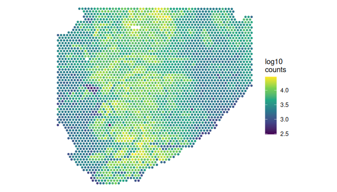
Outlier spots are flagged by their distance from the median in median absolute deviations (MADs), not by fixed thresholds, because a sensible threshold depends on the tissue, the probe panel and the sequencing depth. quickRnaQc.se() has already done this. It set each threshold three MADs from the median, testing library size and detected genes on the low side only (and the mitochondrial share, when there is one, on the high side), and stored the verdict in keep. The thresholds are in the object’s metadata:
thresholds <- metadata(spe)$qc$thresholds
unlist(thresholds)
#>      sum detected
#> 299.5274 224.9087
n_before <- ncol(spe)
n_discard <- sum(!spe$keep)
c(low_sum = sum(spe$sum < thresholds$sum),
    low_detected = sum(spe$detected < thresholds$detected),
    discard = n_discard)
#>      low_sum low_detected      discard
#>            0            1            1
spe <- spe[, spe$keep]
dim(spe)
#> [1] 19338  3394
A large discarded fraction, or discarded spots forming a region, would call for a closer look before dropping them; here 1 of the 3,395 spots is discarded.
Normalisation
Spots differ in library size for technical reasons (capture efficiency, tissue thickness) and biological ones (cell density). The usual choice for Visium is library-size normalisation followed by a log transform. The pooling-based size factors common in single-cell work assume that most genes are not differentially expressed between pools of cells, an assumption that is less safe for spots mixing several cell types. normalizeRnaCounts.se() uses the library sizes as size factors by default, scaled to average 1, and adds the logcounts assay.
spe <- normalizeRnaCounts.se(spe)
summary(spe$sizeFactor)
#>    Min. 1st Qu.  Median    Mean 3rd Qu.    Max.
#> 0.06699 0.41140 0.76224 1.00000 1.38161 4.92577
Feature selection and dimensionality reduction
Highly variable genes carry the structure; the rest add noise. We model the variance of each gene’s log-expression against its mean and mark the 2,000 genes with the largest residual above that trend in rowData(spe)$hvg. Mitochondrial genes, where there are any, are then dropped from the set so that tissue damage does not drive the clustering. This panel has none, so here that step does nothing.
spe <- chooseRnaHvgs.se(spe, top = 2000)
if (any(is_mito)) {
    rowData(spe)$hvg <- rowData(spe)$hvg & !is_mito
}
sum(rowData(spe)$hvg)
#> [1] 2000
hvg_stats <- rowData(spe)[rowData(spe)$hvg, ]
head(rownames(hvg_stats)[order(hvg_stats$residuals, decreasing = TRUE)], 20)
#>  [1] "COL3A1"    "COL1A1"    "COL1A2"    "SERF1B"    "SERF1A"    "MTRNR2L12"
#>  [7] "FN1"       "LYZ"       "TFF3"      "TPM2"      "B2M"       "TFF1"
#> [13] "TNC"       "USP17L8"   "USP17L23"  "TSPAN8"    "COL4A1"    "USP17L5"
#> [19] "IGKC" "SPARC"We keep thirty components, a common default and a generous one for a tissue with a handful of domains. No single component explains much of the variance (the first 4.6%, the second 1.2%), which is usual for spots that each average several cells.
Clustering
Spots are clustered on the principal components with a shared nearest-neighbour graph (Jaccard-weighted) and the Leiden algorithm at resolution 0.5, the settings OSTA uses for its colorectal Visium workflow. The clustering sees expression alone, which turns the spatial plot that follows into a test: if clusters computed without coordinates form coherent regions, they reflect real tissue structure. Spatially aware methods (for example BayesSpace or Banksy) smooth over neighbours and would give cleaner domains, but we would lose that independent check.
spe <- clusterGraph.se(spe, method = "leiden", resolution = 0.5,
    more.build.args = list(weight.scheme = "jaccard"),
    output.name = "cluster")
table(spe$cluster)
#>
#>    1    2    3    4    5
#>  716  740  721 1028  189
spot_plot(spe, spe$cluster, "Cluster") +
    guides(colour = guide_legend(override.aes = list(size = 3)))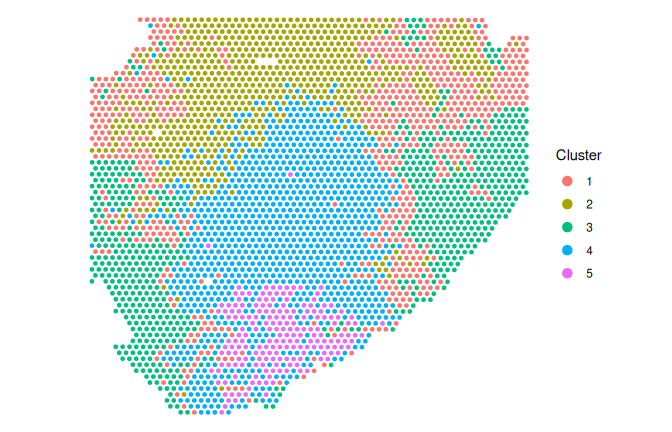
spe <- runUmap.se(spe)
plotReducedDim(spe, "UMAP", colour_by = "cluster")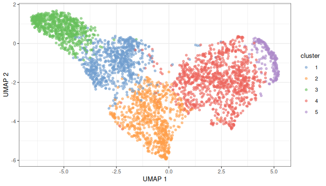
What the clusters are
Marker genes tell us what each cluster is. scoreMarkers.se() compares each cluster with every other one and summarises the pairwise effect sizes for each gene: Cohen’s d (the difference in mean log-expression in standard deviations), the AUC (the probability that a spot in the cluster has higher expression than a spot in the other), and the differences in mean expression and in the proportion of spots where the gene is detected. Genes are ranked by Cohen’s d averaged over the comparisons. Here effect sizes are a better summary than p-values. The clusters were defined from these same expression values, so a test for differences between them is circular, and its p-values would not mean what they usually do.
markers <- scoreMarkers.se(spe, groups = spe$cluster)
top_markers <- vapply(markers, function(m) {
    paste(head(rownames(m), 8), collapse = ", ")
}, "")
tibble::tibble(cluster = names(top_markers), top_markers = top_markers)
#> # A tibble: 5 × 2
#>   cluster top_markers
#>   <chr>   <chr>
#> 1 1       SERF1A, MTRNR2L12, COL1A2, COL3A1, FAM153B, SERF1B, SLC25A5, ANP32E
#> 2 2       COL3A1, COL1A2, COL1A1, FN1, GAGE12J, FKBP10, POLD2, TPM2
#> 3 3       SERF1A, SERF1B, FAM153B, USP17L23, USP17L8, USP17L5, USP17L3, USP17L15
#> 4 4       ACTG1, S100A6, LYZ, UBC, REEP5, HOXB6, HOXB3, TFF3
#> 5 5       B2M, S100A6, TSPAN8, TFF3, LYZ, EPCAM, HSPA8, CEACAM5
Some clusters are led by members of multi-copy gene families, such as SERF1A and SERF1B, FAM153B, the USP17L genes and MTRNR2L12, rather than by genes that mark a cell type. Each of these families has several near-identical copies in the genome, so a probe, or a read, may not be specific to one of them, and the MTRNR2L genes are also close copies of the mitochondrial rRNA gene MT-RNR2. Their signal may therefore be partly technical (this is unverified). The pattern is easier to see in a per-cluster summary of the number of spots, their median depth, the median share of each spot’s counts that goes to these families, and the mean log-expression of an epithelial and a stromal marker:
multicopy <- grepl("^(SERF1|USP17L|FAM153|MTRNR2L|TAF11L|GAGE|CT45A)",
    rownames(spe))
sum(multicopy)
#> [1] 47
clusters <- factor(spe$cluster)
per_cluster <- function(v, f = median) as.vector(tapply(v, clusters, f))
cluster_summary <- tibble::tibble(
    cluster = levels(clusters),
    spots = per_cluster(spe$sum, length),
    median_counts = per_cluster(spe$sum),
    median_genes = per_cluster(spe$detected),
    multicopy_share = round(per_cluster(
        colSums(counts(spe)[multicopy, ]) / spe$sum), 2),
    EPCAM = round(per_cluster(logcounts(spe)["EPCAM", ], mean), 2),
    COL1A1 = round(per_cluster(logcounts(spe)["COL1A1", ], mean), 2)
)
cluster_summary
#> # A tibble: 5 × 7
#>   cluster spots median_counts median_genes multicopy_share EPCAM COL1A1
#>   <chr>   <int>         <dbl>        <dbl>           <dbl> <dbl>  <dbl>
#> 1 1         716         2717         1327             0.17  1.09   2.49
#> 2 2         740         7222.        2926.            0.12  1.45   3.34
#> 3 3         721         1839          868             0.26  0.86   1.98
#> 4 4        1028         6712.        2800             0.1   1.91   2.64
#> 5 5         189        12202         4218             0.08  2.48   1.51
epi <- cluster_summary$cluster[which.max(cluster_summary$EPCAM)]
stroma <- cluster_summary$cluster[which.max(cluster_summary$COL1A1)]
shallow <- cluster_summary$cluster[which.min(cluster_summary$median_counts)]
deepest <- cluster_summary$cluster[which.max(cluster_summary$median_counts)]
The top of the ranking for the most epithelial cluster (highest mean EPCAM) shows the statistics behind it: the mean log-expression and detected proportion in the cluster, then the mean Cohen’s d and AUC against the other clusters.
previewMarkers(markers[[epi]], rows = 8, columns = c("mean", "detected",
    d = "cohens.d.mean", auc = "auc.mean"))
#> DataFrame with 8 rows and 4 columns
#>              mean  detected         d       auc
#>         <numeric> <numeric> <numeric> <numeric>
#> B2M       3.12976  1.000000   1.81411  0.893152
#> S100A6    6.42869  1.000000   1.61075  0.860202
#> TSPAN8    3.34023  1.000000   1.58044  0.868286
#> TFF3      3.59478  1.000000   1.47544  0.847131
#> LYZ       4.28664  1.000000   1.41643  0.837357
#> EPCAM     2.48177  1.000000   1.41317  0.816768
#> HSPA8     2.56627  1.000000   1.40371  0.820702
#> CEACAM5   1.78339  0.957672   1.37423  0.821181
To pin the clusters down, we plot known markers of the colonic mucosa: EPCAM for epithelium, MUC2 for goblet cells and their mucin, CA1 for the absorptive colonocytes that line normal colonic epithelium, COL1A1 for stroma and PTPRC for immune cells. SERF1A stands in for the multi-copy families. Their expression levels differ widely, so each gene is coloured relative to its own maximum:
genes <- intersect(c("EPCAM", "MUC2", "CA1", "COL1A1", "PTPRC", "SERF1A"),
    rownames(spe))
long <- do.call(rbind, lapply(genes, function(g) {
    v <- logcounts(spe)[g, ]
    cbind(spot_coords(spe), gene = g, relative = v / max(v))
}))
ggplot(long, aes(x, y, colour = relative)) +
    geom_point(size = 0.6) +
    scale_colour_viridis_c(labels = scales::percent) +
    scale_y_reverse() +
    coord_fixed() +
    facet_wrap(~ gene) +
    labs(x = NULL, y = NULL, colour = "Share of\nmaximum") +
    theme_void()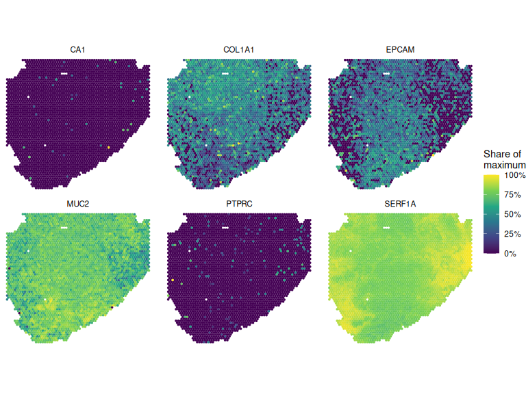
plotDots(spe, features = genes, group = "cluster")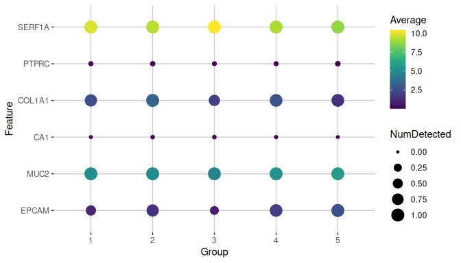
Read together, the plots and the summary suggest three kinds of spot:
- Epithelium. The cluster with the highest
EPCAM(cluster 5) has epithelial and secretory genes among its top markers (B2M,S100A6,TSPAN8,TFF3,LYZ,EPCAM,HSPA8,CEACAM5), and the deepest spots. - Stroma. The cluster with the highest
COL1A1(cluster 2) is led by collagens and other stromal and extracellular-matrix genes (COL3A1,COL1A2,COL1A1,FN1,GAGE12J,FKBP10). - Shallow spots. The cluster with the fewest counts per spot (cluster 3) is led by the multi-copy families (
SERF1A,SERF1B,FAM153B,USP17L23,USP17L8,USP17L5), which take 26% of a typical spot’s counts there. These spots lie along the edges of the section, where the library-size map is darkest, and the cluster may reflect capture depth more than a cell type.
The section as a whole does not look like normal colonic mucosa. MUC2 is detected throughout (in 100% of spots), while the markers of absorptive colonocytes (CA1, FABP1, SLC26A3, AQP8) are almost absent (each detected in at most 1% of spots), and so is the immune marker PTPRC (4%). That would fit a mucin-rich lesion, but the histology is not recorded, so it remains a hypothesis: the H&E image of the section (an auxiliary file of a few gigabytes) is the place to check it.
So the expression clusters do form regions on the tissue, which suggests real structure. But they separate spots by depth and by a few gene families as well as by tissue compartment. Two next steps would sharpen them: drop the multi-copy families from the highly variable genes and recluster, and compare the regions with the H&E image.
Where to go from here
Other Vanderbilt Visium files cover more colon lesions (candidates above). You can read several, give each its file ID, and combine them in one MultiAssayExperiment, then integrate them with batch correction (for example scrapper’s correctMnn.se()) before clustering them together.
The participant also has single-cell RNA-seq (Level 3 count matrices). Cell types from those can be used to deconvolve the spots, for example with SPOTlight.
For spatially smoothed domains there are BayesSpace and Banksy; for spatially variable genes, nnSVG.
Beyond this participant, htan_files() and the clinical tables find comparable sections from other atlases, for example premalignant versus invasive tissue.
Notes on reproducibility
The metadata release is pinned (htan_con("r7")), and the file is identified by its HTAN ID and checked against its md5. The random steps (PCA, clustering, UMAP) use scrapper’s fixed default seeds, so on a given platform and set of package versions they give the same result on every run without set.seed(). Across versions and platforms the details can change: builds of this vignette with different scrapper releases and numerical libraries have given five or six clusters. That is why every result quoted in the text above is computed from the output rather than written in by hand. The software versions are listed below.
The file’s content on Synapse is not pinned. If the center replaced the file, the md5 check would fail rather than silently give a different result.
Session information
sessionInfo()
#> R version 4.6.1 (2026-06-24)
#> Platform: x86_64-pc-linux-gnu
#> Running under: Ubuntu 24.04.5 LTS
#>
#> Matrix products: default
#> BLAS:   /usr/lib/x86_64-linux-gnu/openblas-pthread/libblas.so.3
#> LAPACK: /usr/lib/x86_64-linux-gnu/openblas-pthread/libopenblasp-r0.3.26.so;  LAPACK version 3.12.0
#>
#> locale:
#>  [1] LC_CTYPE=en_US.UTF-8       LC_NUMERIC=C
#>  [3] LC_TIME=en_US.UTF-8        LC_COLLATE=en_US.UTF-8
#>  [5] LC_MONETARY=en_US.UTF-8    LC_MESSAGES=en_US.UTF-8
#>  [7] LC_PAPER=en_US.UTF-8       LC_NAME=C
#>  [9] LC_ADDRESS=C               LC_TELEPHONE=C
#> [11] LC_MEASUREMENT=en_US.UTF-8 LC_IDENTIFICATION=C
#>
#> time zone: Etc/UTC
#> tzcode source: system (glibc)
#>
#> attached base packages:
#> [1] stats4    stats     graphics  grDevices utils     datasets  methods
#> [8] base
#>
#> other attached packages:
#>  [1] dplyr_1.2.1                 HTAN_0.99.1
#>  [3] scrapper_1.7.9              scater_1.41.2
#>  [5] ggplot2_4.0.3               scuttle_1.23.2
#>  [7] SpatialExperiment_1.23.0    SingleCellExperiment_1.35.2
#>  [9] SummarizedExperiment_1.43.0 Biobase_2.73.2
#> [11] GenomicRanges_1.65.4        Seqinfo_1.3.2
#> [13] IRanges_2.47.5              S4Vectors_0.51.10
#> [15] BiocGenerics_0.59.12        generics_0.1.4
#> [17] MatrixGenerics_1.25.0       matrixStats_1.5.0
#>
#> loaded via a namespace (and not attached):
#>  [1] tidyselect_1.2.1            viridisLite_0.4.3
#>  [3] vipor_0.4.7                 farver_2.1.2
#>  [5] blob_1.3.0                  filelock_1.0.3
#>  [7] viridis_0.6.5               S7_0.2.2
#>  [9] fastmap_1.2.0               BiocFileCache_3.3.0
#> [11] duckdb_1.5.6                digest_0.6.39
#> [13] rsvd_1.0.5                  lifecycle_1.0.5
#> [15] RSQLite_3.53.3              magrittr_2.0.5
#> [17] compiler_4.6.1              rlang_1.3.0
#> [19] tools_4.6.1                 utf8_1.2.6
#> [21] yaml_2.3.12                 knitr_1.52
#> [23] labeling_0.4.3              S4Arrays_1.13.2
#> [25] bit_4.6.0                   curl_8.1.0
#> [27] reticulate_1.47.0           DelayedArray_0.39.8
#> [29] RColorBrewer_1.1-3          abind_1.4-8
#> [31] BiocParallel_1.47.0         withr_3.0.3
#> [33] purrr_1.2.2                 grid_4.6.1
#> [35] beachmat_2.29.3             Rhdf5lib_2.1.0
#> [37] scales_1.4.0                MultiAssayExperiment_1.39.1
#> [39] cli_3.6.6                   rmarkdown_2.32
#> [41] otel_0.2.0                  rjson_0.2.23
#> [43] rhdf5_2.57.20               DBI_1.3.0
#> [45] ggbeeswarm_0.7.3            cachem_1.1.0
#> [47] parallel_4.6.1              XVector_0.53.0
#> [49] vctrs_0.7.3                 Matrix_1.7-6
#> [51] jsonlite_2.0.0              BiocSingular_1.29.2
#> [53] BiocNeighbors_2.7.3         bit64_4.8.6
#> [55] ggrepel_0.9.8               irlba_2.4.1
#> [57] beeswarm_0.4.0              magick_2.9.1
#> [59] glue_1.8.1                  codetools_0.2-20
#> [61] gtable_0.3.6                ScaledMatrix_1.21.0
#> [63] tibble_3.3.1                pillar_1.11.1
#> [65] rhdf5filters_1.25.4         htmltools_0.5.9
#> [67] R6_2.6.1                    dbplyr_2.6.0
#> [69] httr2_1.3.0                 evaluate_1.0.5
#> [71] lattice_0.23-1              png_0.1-9
#> [73] memoise_2.0.1               Rcpp_1.1.2
#> [75] gridExtra_2.3.1             SparseArray_1.13.4
#> [77] anndataR_1.3.2              xfun_0.61
#> [79] pkgconfig_2.0.3