Clustering

Experimental background

The data we are going to use are from deRisi et al.. From their abstract:

DNA microarrays containing virtually every gene of Saccharomyces cerevisiae were used to carry out a comprehensive investigation of the temporal program of gene expression accompanying the metabolic shift from fermentation to respiration. The expression profiles observed for genes with known metabolic functions pointed to features of the metabolic reprogramming that occur during the diauxic shift, and the expression patterns of many previously uncharacterized genes provided clues to their possible functions.

These data are available from NCBI GEO as GSE28.

In the case of the baker’s or brewer’s yeast Saccharomyces cerevisiae growing on glucose with plenty of aeration, the diauxic growth pattern is commonly observed in batch culture. During the first growth phase, when there is plenty of glucose and oxygen available, the yeast cells prefer glucose fermentation to aerobic respiration even though aerobic respiration is the more efficient pathway to grow on glucose. This experiment profiles gene expression for 6400 genes over a time course during which the cells are undergoing a diauxic shift.

The data in deRisi et al. have no replicates and are time course data. Sometimes, seeing how groups of genes behave can give biological insight into the experimental system or the function of individual genes. We can use clustering to group genes that have a similar expression pattern over time and then potentially look at the genes that do so.

Our goal, then, is to use kmeans clustering to divide highly variable (informative) genes into groups and then to visualize those groups.

Getting data

These data were deposited at NCBI GEO back in 2002. GEOquery can pull them out easily.

library(GEOquery)

## Loading required package: Biobase

## Loading required package: BiocGenerics

## 
## Attaching package: 'BiocGenerics'

## The following objects are masked from 'package:stats':
## 
##     IQR, mad, sd, var, xtabs

## The following objects are masked from 'package:base':
## 
##     anyDuplicated, append, as.data.frame, basename, cbind, colnames,
##     dirname, do.call, duplicated, eval, evalq, Filter, Find, get, grep,
##     grepl, intersect, is.unsorted, lapply, Map, mapply, match, mget,
##     order, paste, pmax, pmax.int, pmin, pmin.int, Position, rank,
##     rbind, Reduce, rownames, sapply, setdiff, sort, table, tapply,
##     union, unique, unsplit, which.max, which.min

## Welcome to Bioconductor
## 
##     Vignettes contain introductory material; view with
##     'browseVignettes()'. To cite Bioconductor, see
##     'citation("Biobase")', and for packages 'citation("pkgname")'.

## Setting options('download.file.method.GEOquery'='auto')

## Setting options('GEOquery.inmemory.gpl'=FALSE)

gse = getGEO("GSE28")[[1]]

## Found 1 file(s)

## GSE28_series_matrix.txt.gz

class(gse)

## [1] "ExpressionSet"
## attr(,"package")
## [1] "Biobase"

GEOquery is a little dated and was written before the SummarizedExperiment existed. However, Bioconductor makes a conversion from the old ExpressionSet that GEOquery uses to the SummarizedExperiment that we see so commonly used now.

library(SummarizedExperiment)

## Loading required package: MatrixGenerics

## Loading required package: matrixStats

## 
## Attaching package: 'matrixStats'

## The following objects are masked from 'package:Biobase':
## 
##     anyMissing, rowMedians

## 
## Attaching package: 'MatrixGenerics'

## The following objects are masked from 'package:matrixStats':
## 
##     colAlls, colAnyNAs, colAnys, colAvgsPerRowSet, colCollapse,
##     colCounts, colCummaxs, colCummins, colCumprods, colCumsums,
##     colDiffs, colIQRDiffs, colIQRs, colLogSumExps, colMadDiffs,
##     colMads, colMaxs, colMeans2, colMedians, colMins, colOrderStats,
##     colProds, colQuantiles, colRanges, colRanks, colSdDiffs, colSds,
##     colSums2, colTabulates, colVarDiffs, colVars, colWeightedMads,
##     colWeightedMeans, colWeightedMedians, colWeightedSds,
##     colWeightedVars, rowAlls, rowAnyNAs, rowAnys, rowAvgsPerColSet,
##     rowCollapse, rowCounts, rowCummaxs, rowCummins, rowCumprods,
##     rowCumsums, rowDiffs, rowIQRDiffs, rowIQRs, rowLogSumExps,
##     rowMadDiffs, rowMads, rowMaxs, rowMeans2, rowMedians, rowMins,
##     rowOrderStats, rowProds, rowQuantiles, rowRanges, rowRanks,
##     rowSdDiffs, rowSds, rowSums2, rowTabulates, rowVarDiffs, rowVars,
##     rowWeightedMads, rowWeightedMeans, rowWeightedMedians,
##     rowWeightedSds, rowWeightedVars

## The following object is masked from 'package:Biobase':
## 
##     rowMedians

## Loading required package: GenomicRanges

## Loading required package: stats4

## Loading required package: S4Vectors

## 
## Attaching package: 'S4Vectors'

## The following objects are masked from 'package:base':
## 
##     expand.grid, I, unname

## Loading required package: IRanges

## Loading required package: GenomeInfoDb

gse = as(gse, "SummarizedExperiment")
gse

## class: SummarizedExperiment 
## dim: 6400 7 
## metadata(3): experimentData annotation protocolData
## assays(1): exprs
## rownames(6400): 1 2 ... 6399 6400
## rowData names(20): ID ORF ... FAILED IS_CONTAMINATED
## colnames(7): GSM887 GSM888 ... GSM892 GSM893
## colData names(33): title geo_accession ... supplementary_file
##   data_row_count

Taking a quick look at the colData(), it might be that we want to reorder the columns a bit.

colData(gse)$title

## [1] "diauxic shift timecourse: 15.5 hr" "diauxic shift timecourse: 0 hr"   
## [3] "diauxic shift timecourse: 18.5 hr" "diauxic shift timecourse: 9.5 hr" 
## [5] "diauxic shift timecourse: 11.5 hr" "diauxic shift timecourse: 13.5 hr"
## [7] "diauxic shift timecourse: 20.5 hr"

So, we can reorder by hand to get the time course correct:

gse = gse[, c(2,4,5,6,1,3,7)]

sds = apply(assays(gse)[[1]], 1, sd)
hist(sds)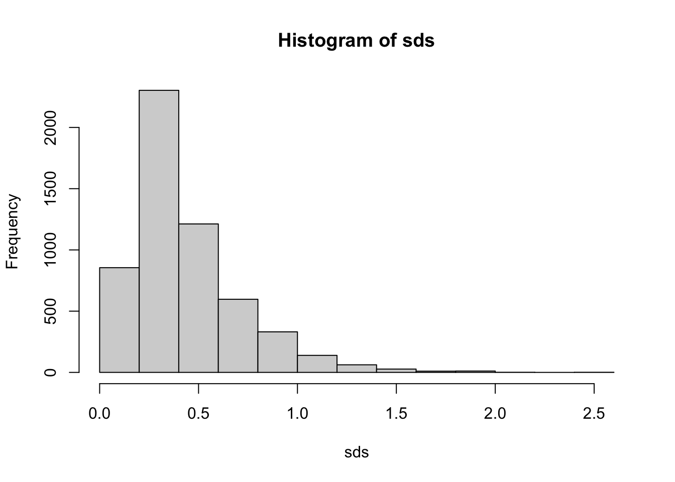

Examining the plot, we can see that the most highly variable genes have an sd > 0.8 or so (arbitrary). We can, for convenience, create a new SummarizedExperiment that contains only our most highly variable genes.

idx = sds>0.8 & !is.na(sds)
gse_sub = gse[idx,]

Now, gse_sub contains a subset of our data.

The kmeans function takes a matrix and the number of clusters as arguments.

k = 4
km = kmeans(assays(gse_sub)[[1]], 4)

The km kmeans result contains a vector, km$cluster, which gives the cluster associated with each gene. We can plot the genes for each cluster to see how these different genes behave.

expression_values = assays(gse_sub)[[1]]
par(mfrow=c(2,2), mar=c(3,4,1,2)) # this allows multiple plots per page
for(i in 1:k) {
    matplot(t(expression_values[km$cluster==i, ]), type='l', ylim=c(-3,3),
            ylab = paste("cluster", i))
}

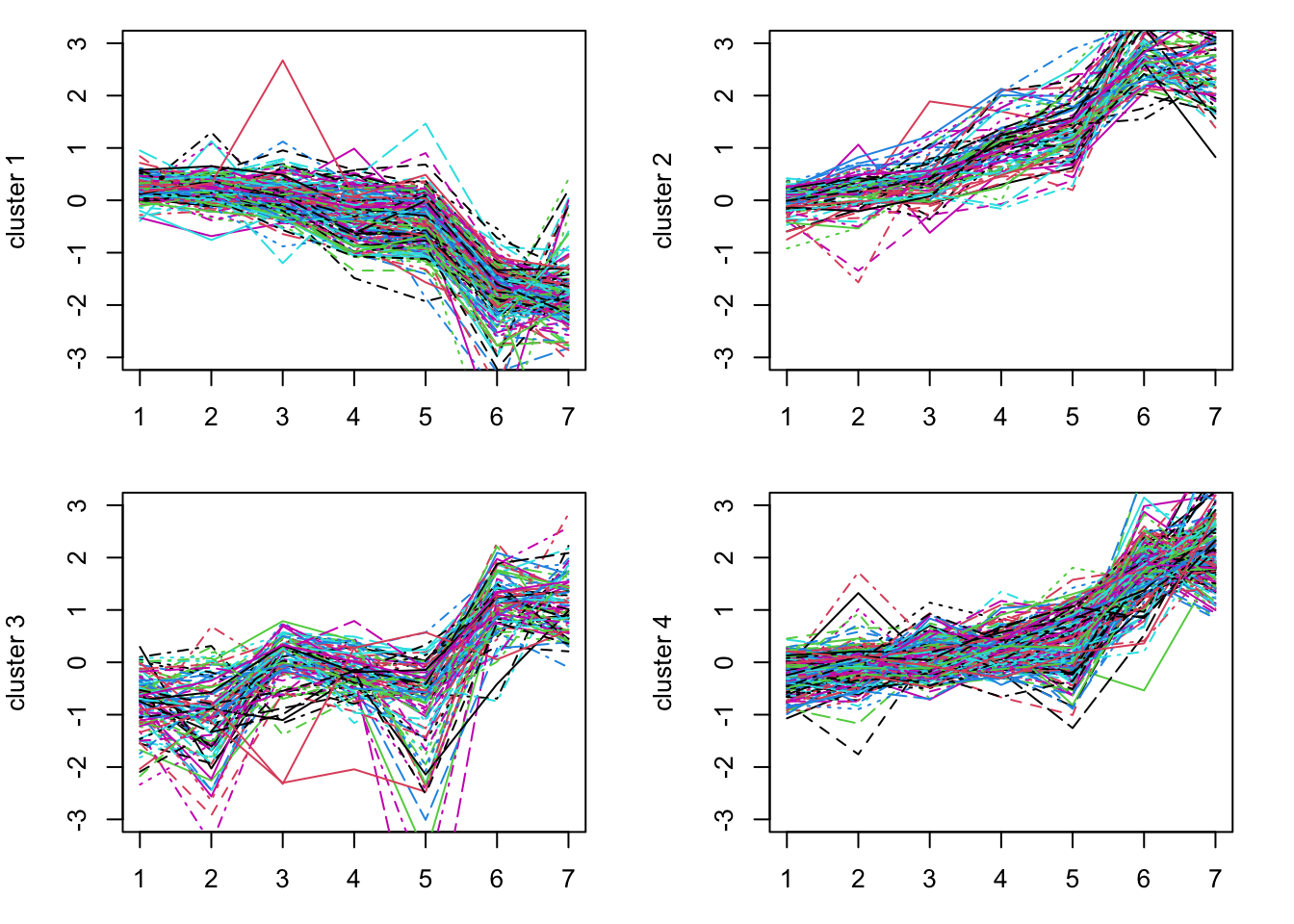
Try this with different size k. Perhaps go back to choose more genes (using a smaller cutoff for sd).