Accessing and working with public omics data
The data
The data we are going to access are from this paper.
Background: The tumor microenvironment is an important factor in cancer immunotherapy response. To further understand how a tumor affects the local immune system, we analyzed immune gene expression differences between matching normal and tumor tissue.Methods: We analyzed public and new gene expression data from solid cancers and isolated immune cell populations. We also determined the correlation between CD8, FoxP3 IHC, and our gene signatures.Results: We observed that regulatory T cells (Tregs) were one of the main drivers of immune gene expression differences between normal and tumor tissue. A tumor-specific CD8 signature was slightly lower in tumor tissue compared with normal of most (12 of 16) cancers, whereas a Treg signature was higher in tumor tissue of all cancers except liver. Clustering by Treg signature found two groups in colorectal cancer datasets. The high Treg cluster had more samples that were consensus molecular subtype 1/4, right-sided, and microsatellite-instable, compared with the low Treg cluster. Finally, we found that the correlation between signature and IHC was low in our small dataset, but samples in the high Treg cluster had significantly more CD8+ and FoxP3+ cells compared with the low Treg cluster.Conclusions: Treg gene expression is highly indicative of the overall tumor immune environment.Impact: In comparison with the consensus molecular subtype and microsatellite status, the Treg signature identifies more colorectal tumors with high immune activation that may benefit from cancer immunotherapy.
In this little exercise, we will:
- Access public omics data using the GEOquery package
- Get an opportunity to work with another SummarizedExperiment object.
- Perform a simple unsupervised analysis to visualize these public data.
GEOquery to multidimensional scaling
Use the GEOquery package to fetch data about GSE103512.
library(GEOquery)
gse = getGEO("GSE103512")[[1]]
The first step, a detail, is to convert from the older Bioconductor
data structure (GEOquery was written in 2007), the
ExpressionSet, to the newer
SummarizedExperiment.
library(SummarizedExperiment)## Loading required package: MatrixGenerics## Loading required package: matrixStats##
## Attaching package: 'matrixStats'## The following objects are masked from 'package:Biobase':
##
## anyMissing, rowMedians##
## Attaching package: 'MatrixGenerics'## The following objects are masked from 'package:matrixStats':
##
## colAlls, colAnyNAs, colAnys, colAvgsPerRowSet, colCollapse,
## colCounts, colCummaxs, colCummins, colCumprods, colCumsums,
## colDiffs, colIQRDiffs, colIQRs, colLogSumExps, colMadDiffs,
## colMads, colMaxs, colMeans2, colMedians, colMins, colOrderStats,
## colProds, colQuantiles, colRanges, colRanks, colSdDiffs, colSds,
## colSums2, colTabulates, colVarDiffs, colVars, colWeightedMads,
## colWeightedMeans, colWeightedMedians, colWeightedSds,
## colWeightedVars, rowAlls, rowAnyNAs, rowAnys, rowAvgsPerColSet,
## rowCollapse, rowCounts, rowCummaxs, rowCummins, rowCumprods,
## rowCumsums, rowDiffs, rowIQRDiffs, rowIQRs, rowLogSumExps,
## rowMadDiffs, rowMads, rowMaxs, rowMeans2, rowMedians, rowMins,
## rowOrderStats, rowProds, rowQuantiles, rowRanges, rowRanks,
## rowSdDiffs, rowSds, rowSums2, rowTabulates, rowVarDiffs, rowVars,
## rowWeightedMads, rowWeightedMeans, rowWeightedMedians,
## rowWeightedSds, rowWeightedVars## The following object is masked from 'package:Biobase':
##
## rowMedians## Loading required package: GenomicRanges## Loading required package: stats4## Loading required package: S4Vectors##
## Attaching package: 'S4Vectors'## The following objects are masked from 'package:base':
##
## expand.grid, I, unname## Loading required package: IRanges## Loading required package: GenomeInfoDbse = as(gse, "SummarizedExperiment")Examine two variables of interest, cancer type and tumor/normal status.
with(colData(se),table(`cancer.type.ch1`,`normal.ch1`))## normal.ch1
## cancer.type.ch1 no yes
## BC 65 10
## CRC 57 12
## NSCLC 60 9
## PCA 60 7Filter gene expression by variance to find most informative genes.
sds = apply(assay(se, 'exprs'),1,sd)
dat = assay(se, 'exprs')[order(sds,decreasing = TRUE)[1:500],]
Perform multidimensional scaling and prepare for plotting. We will be using ggplot2, so we need to make a data.frame before plotting.
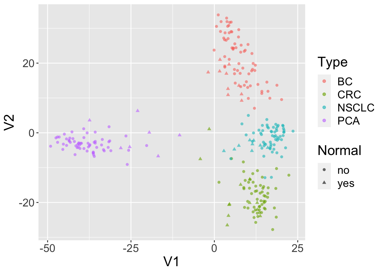
mdsvals = cmdscale(dist(t(dat)))
mdsvals = as.data.frame(mdsvals)
mdsvals$Type=factor(colData(se)[,'cancer.type.ch1'])
mdsvals$Normal = factor(colData(se)[,'normal.ch1'])
And do the plot.
library(ggplot2)
ggplot(mdsvals, aes(x=V1,y=V2,shape=Normal,color=Type)) +
    geom_point( alpha=0.6) + theme(text=element_text(size = 18))