Data exploration and univariate statistics
Behavioral Risk Factor Surveillance System
We will explore a subset of data collected by the CDC through its extensive Behavioral Risk Factor Surveillance System ([BRFSS][]) telephone survey. Check out the link for more information. We’ll look at a subset of the data.
First, we need to get the data. Either download the data from THIS LINK or have R do it directly from the command-line (preferred):
download.file('https://raw.githubusercontent.com/seandavi/ITR/master/BRFSS-subset.csv',
              destfile = 'BRFSS-subset.csv')
path <- file.choose() # look for BRFSS-subset.csvstopifnot(file.exists(path))
brfss <- read.csv(path)Learn about the data
Using the data exploration techniques you have seen to explore the brfss dataset.
- summary()
- dim()
- colnames()
- head()
- tail()
- class()
- View()
You may want to investigate individual columns visually using
plotting like hist(). For categorical data, consider using
something like table().
Clean data
R read Year as an integer value, but it’s
really a factor
brfss$Year <- factor(brfss$Year)Weight in 1990 vs. 2010 Females
- Create a subset of the data
brfssFemale <- brfss[brfss$Sex == "Female",]
summary(brfssFemale)
## Age Weight Sex Height
## Min. :18.00 Min. : 36.29 Length:12039 Min. :105.0
## 1st Qu.:37.00 1st Qu.: 57.61 Class :character 1st Qu.:157.5
## Median :52.00 Median : 65.77 Mode :character Median :163.0
## Mean :51.92 Mean : 69.05 Mean :163.3
## 3rd Qu.:67.00 3rd Qu.: 77.11 3rd Qu.:168.0
## Max. :99.00 Max. :272.16 Max. :200.7
## NA's :103 NA's :560 NA's :140
## Year
## 1990:5718
## 2010:6321
##
##
##
##
## - Visualize
plot(Weight ~ Year, brfssFemale)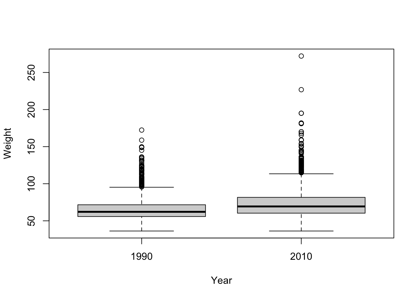
- Statistical test
t.test(Weight ~ Year, brfssFemale)##
## Welch Two Sample t-test
##
## data: Weight by Year
## t = -27.133, df = 11079, p-value < 2.2e-16
## alternative hypothesis: true difference in means between group 1990 and group 2010 is not equal to 0
## 95 percent confidence interval:
## -8.723607 -7.548102
## sample estimates:
## mean in group 1990 mean in group 2010
## 64.81838 72.95424Weight and height in 2010 Males
- Create a subset of the data
brfss2010Male <- subset(brfss,  Year == 2010 & Sex == "Male")
summary(brfss2010Male)
## Age Weight Sex Height Year
## Min. :18.00 Min. : 36.29 Length:3679 Min. :135 1990: 0
## 1st Qu.:45.00 1st Qu.: 77.11 Class :character 1st Qu.:173 2010:3679
## Median :57.00 Median : 86.18 Mode :character Median :178
## Mean :56.25 Mean : 88.85 Mean :178
## 3rd Qu.:68.00 3rd Qu.: 99.79 3rd Qu.:183
## Max. :99.00 Max. :278.96 Max. :218
## NA's :30 NA's :49 NA's :31- Visualize the relationship
hist(brfss2010Male$Weight)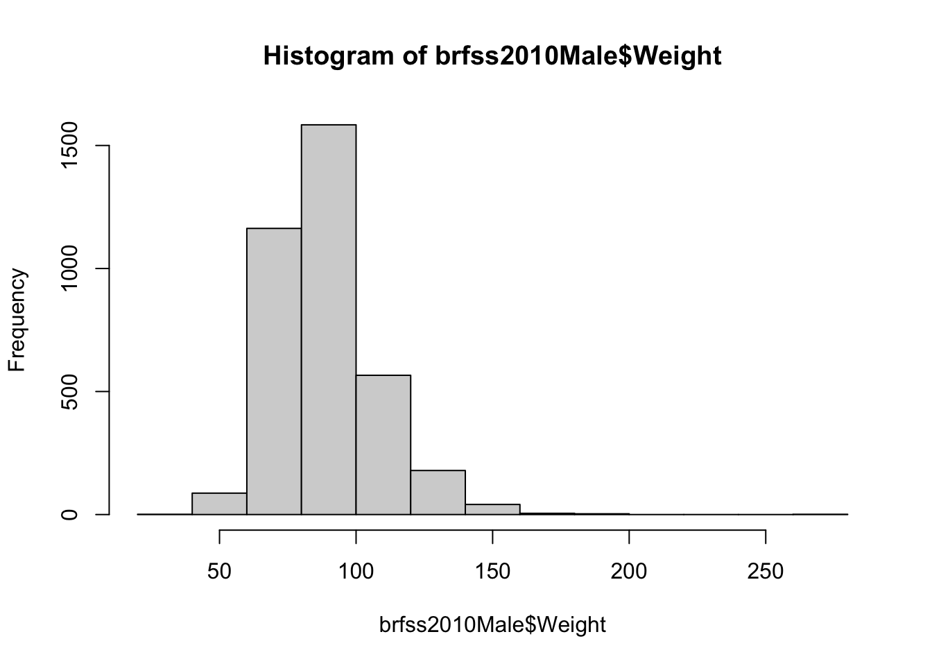
hist(brfss2010Male$Height)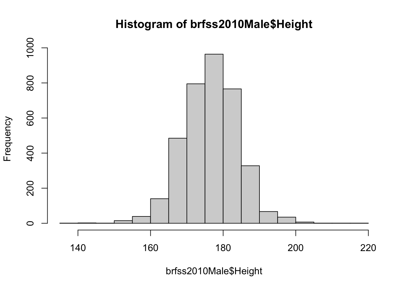
plot(Weight ~ Height, brfss2010Male)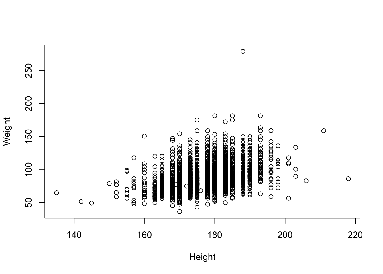
- Fit a linear model (regression)
fit <- lm(Weight ~ Height, brfss2010Male)
fit
##
## Call:
## lm(formula = Weight ~ Height, data = brfss2010Male)
##
## Coefficients:
## (Intercept) Height
## -86.8747 0.9873Summarize as ANOVA table
anova(fit)## Analysis of Variance Table
##
## Response: Weight
## Df Sum Sq Mean Sq F value Pr(>F)
## Height 1 197664 197664 693.8 < 2.2e-16 ***
## Residuals 3617 1030484 285
## ---
## Signif. codes: 0 '***' 0.001 '**' 0.01 '*' 0.05 '.' 0.1 ' ' 1- Plot points, superpose fitted regression line; where am I?
plot(Weight ~ Height, brfss2010Male)
abline(fit, col="blue", lwd=2)
# Substitute your own weight and height...
points(73 * 2.54, 178 / 2.2, col="red", cex=4, pch=20)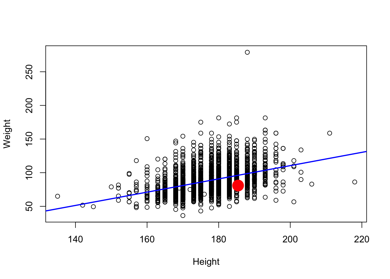
- Class and available ‘methods’
class(fit)                 # 'noun'
methods(class=class(fit)) # 'verb'- Diagnostics
plot(fit)
# Note that the "plot" above does not have a ".lm"
# However, R will use "plot.lm". Why?
?plot.lm