Data Input and Manipulation Exercises

Behavioral Risk Factor Surveillance System

We will explore a subset of data collected by the CDC through its extensive Behavioral Risk Factor Surveillance System (BRFSS) telephone survey. Check out the link for more information. We’ll look at a subset of the data.

First, we need to get the data. Either download the data from THIS LINK or have R do it directly from the command-line (preferred):

download.file('https://raw.githubusercontent.com/seandavi/ITR/master/BRFSS-subset.csv',
              destfile = 'BRFSS-subset.csv')

You can check to see the file using the Rstudio file panel or get a directory listing using dir()

Use file.choose() to find the path to the file ‘BRFSS-subset.csv’. This is a quick-and-dirty to find a file on the computer. Store the file location into a variable called path.
```
path <- file.choose()
```

Read the data into R using read.csv(), assigning to a variable brfss. Note that you can use the path variable in read.csv().
```
brfss <- read.csv(path)
```
Use command like class(), head(), dim(), summary() to explore the data.
- What variables have been measured?
- Can you guess at the units used for, e.g., Weight and Height?
```
class(brfss)
head(brfss)
dim(brfss)
summary(brfss)
```

Use the $ operator to extract the Sex column, and summarize the number of males and females in the survey using table(brfss$Sex). Do the same for Year, and for both Sex and Year.

table(brfss$Sex)

## 
## Female   Male 
##  12039   7961

table(brfss$Year)

## 
##  1990  2010 
## 10000 10000

table(brfss$Sex, brfss$Year)

##         
##          1990 2010
##   Female 5718 6321
##   Male   4282 3679

with(brfss, table(Sex, Year))                # same, but easier

##         Year
## Sex      1990 2010
##   Female 5718 6321
##   Male   4282 3679

Use aggregate() to summarize the mean weight of each group. What about the median weight of each group? What about the number of observations in each group?

with(brfss, aggregate(Weight, list(Year, Sex), mean, na.rm=TRUE))

##   Group.1 Group.2        x
## 1    1990  Female 64.81838
## 2    2010  Female 72.95424
## 3    1990    Male 81.17999
## 4    2010    Male 88.84657

with(brfss, aggregate(Weight, list(Year=Year, Sex=Sex), mean, na.rm=TRUE))

##   Year    Sex        x
## 1 1990 Female 64.81838
## 2 2010 Female 72.95424
## 3 1990   Male 81.17999
## 4 2010   Male 88.84657

Use a formula and the aggregate() function to describe the relationship between Year, Sex, and Weight

aggregate(Weight ~ Year + Sex, brfss, mean)  # same, but more informative

##   Year    Sex   Weight
## 1 1990 Female 64.81838
## 2 2010 Female 72.95424
## 3 1990   Male 81.17999
## 4 2010   Male 88.84657

aggregate(. ~ Year + Sex, brfss, mean)       # all variables

##   Year    Sex      Age   Weight   Height
## 1 1990 Female 46.09153 64.84333 163.2914
## 2 2010 Female 57.07807 73.03178 163.2469
## 3 1990   Male 43.87574 81.19496 178.2242
## 4 2010   Male 56.25465 88.91136 178.0139

Create a subset of the data consisting of only the 1990 observations. Perform a t-test comparing the weight of males and females (“‘Weight’ as a function of ‘Sex’”, Weight ~ Sex)

brfss_1990 = brfss[brfss$Year == 1990,]
t.test(Weight ~ Sex, brfss_1990)

## 
##  Welch Two Sample t-test
## 
## data:  Weight by Sex
## t = -58.734, df = 9214, p-value < 2.2e-16
## alternative hypothesis: true difference in means between group Female and group Male is not equal to 0
## 95 percent confidence interval:
##  -16.90767 -15.81554
## sample estimates:
## mean in group Female   mean in group Male 
##             64.81838             81.17999

t.test(Weight ~ Sex, brfss, subset = Year == 1990)

## 
##  Welch Two Sample t-test
## 
## data:  Weight by Sex
## t = -58.734, df = 9214, p-value < 2.2e-16
## alternative hypothesis: true difference in means between group Female and group Male is not equal to 0
## 95 percent confidence interval:
##  -16.90767 -15.81554
## sample estimates:
## mean in group Female   mean in group Male 
##             64.81838             81.17999

What about differences between weights of males (or females) in 1990 versus 2010? Check out the help page ?t.test.formula. Is there a way of performing a t-test on brfss without explicitly creating the object brfss_1990?

Use boxplot() to plot the weights of the Male individuals. Can you transform weight, e.g., sqrt(Weight) ~ Year? Interpret the results. Do similar boxplots for the t-tests of the previous question.
```
boxplot(Weight ~ Year, brfss, subset = Sex == "Male",
        main="Males")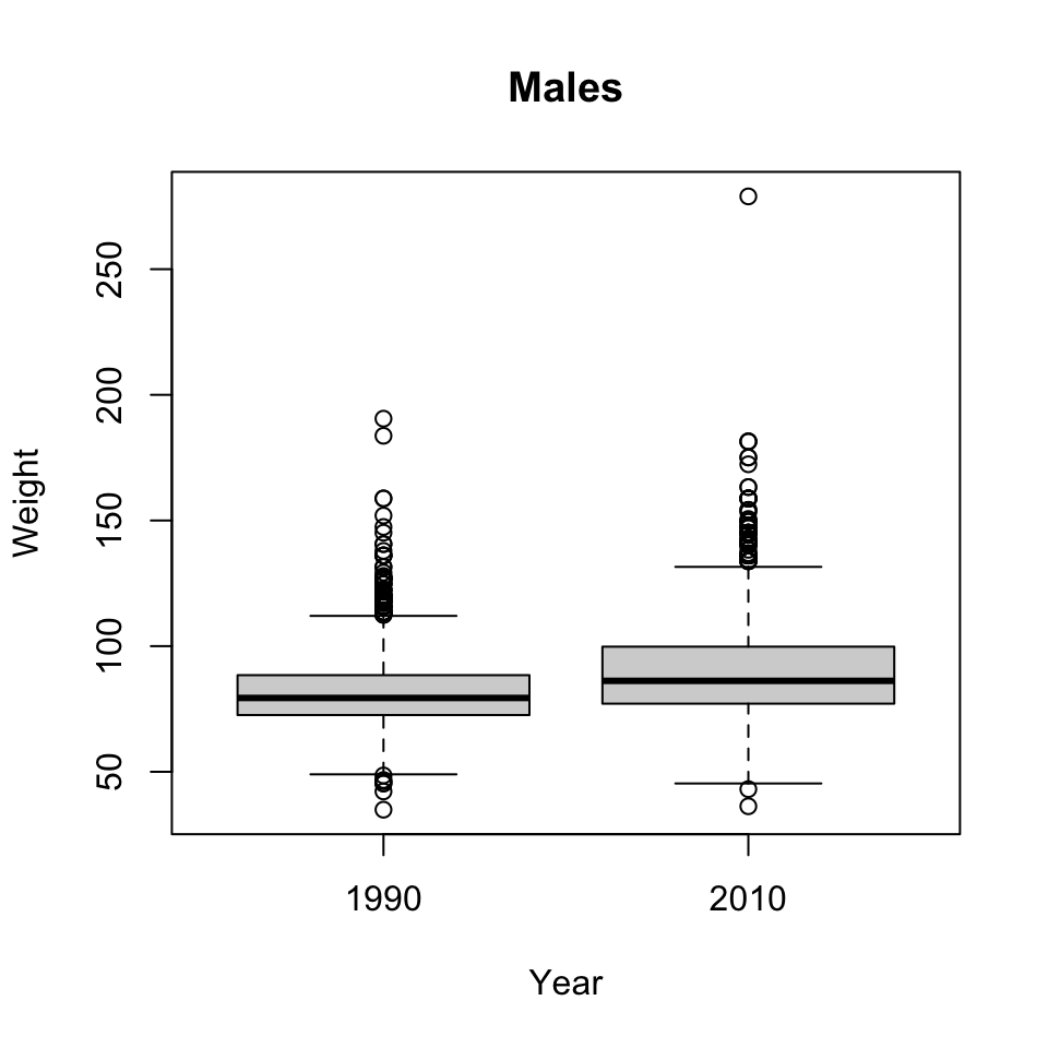
```

Use hist() to plot a histogram of weights of the 1990 Female individuals.

hist(brfss_1990[brfss_1990$Sex == "Female", "Weight"],
     main="Females, 1990", xlab="Weight" )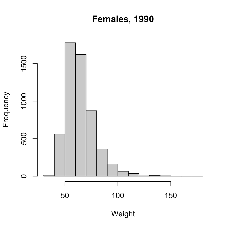

BONUS: ggplot2

library(ggplot2)

http://docs.ggplot2.org

‘Grammar of graphics’

Specify data and ‘aesthetics’ (aes()) to be plotted
Add layers (geom_*()) of information

Clean it by coercing Year to factor. A factor is a categorical variable. In this case, our data have only two years represented, so we will treat these two years as “groups” or categories.

brfss$Year <- factor(brfss$Year)

Let’s make a couple of subsets of data to work with. First, let’s subset to get only males in 2010.

brfss2010Male = subset(brfss,Sex=='Male' & Year=='2010')

and make an “only female” subset.

brfssFemale = subset(brfss,Sex=='Female')

```r
ggplot(brfss2010Male, aes(x=Height, y=Weight)) +
    geom_point() +
    geom_smooth(method="lm")
```

```
## `geom_smooth()` using formula 'y ~ x'
```

<img src="data_input_and_manipulation_exercises_files/figure-html/unnamed-chunk-4-1.png" width="672" />

Capture a plot and augment it

plt <- ggplot(brfss2010Male, aes(x=Height, y=Weight)) +
    geom_point() +
    geom_smooth(method="lm")
plt + labs(title = "2010 Male")

## `geom_smooth()` using formula 'y ~ x'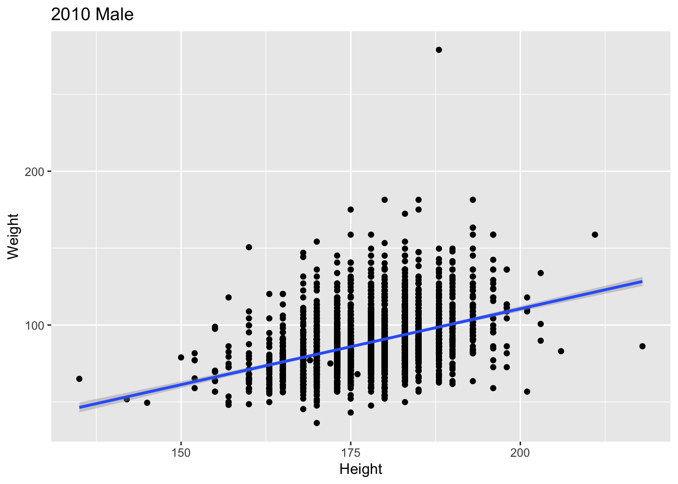

Use facet_*() for layouts

ggplot(brfssFemale, aes(x=Height, y=Weight)) +
    geom_point() + geom_smooth(method="lm") +
    facet_grid(. ~ Year)

## `geom_smooth()` using formula 'y ~ x'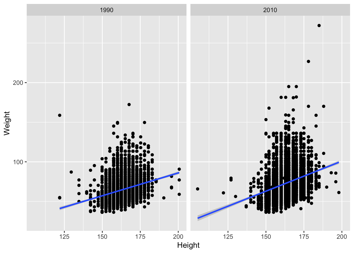

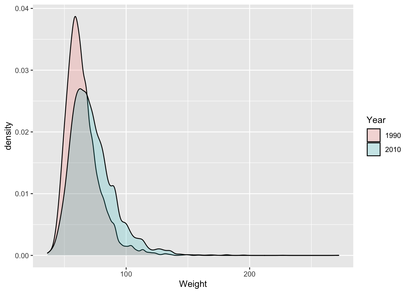
Choose display to emphasize relevant aspects of data

ggplot(brfssFemale, aes(Weight, fill=Year)) +
    geom_density(alpha=.2)