Working with Genomic Ranges
Getting started
Genomic ranges are a way of describing regions on the genome (or any other linear object, such as a transcript, or even a protein). This functionality is typically found in the GenomicRanges package.
library(GenomicRanges)Example GRanges
To get going, we can construct a GRanges object by hand
as an example.
gr <- GRanges(
    seqnames = Rle(c("chr1", "chr2", "chr1", "chr3"), c(1, 3, 2, 4)),
    ranges = IRanges(101:110, end = 111:120, names = head(letters, 10)),
    strand = Rle(strand(c("-", "+", "*", "+", "-")), c(1, 2, 2, 3, 2)),
    score = 1:10,
    GC = seq(1, 0, length=10))
gr
## GRanges object with 10 ranges and 2 metadata columns:
## seqnames ranges strand | score GC
## <Rle> <IRanges> <Rle> | <integer> <numeric>
## a chr1 101-111 - | 1 1.000000
## b chr2 102-112 + | 2 0.888889
## c chr2 103-113 + | 3 0.777778
## d chr2 104-114 * | 4 0.666667
## e chr1 105-115 * | 5 0.555556
## f chr1 106-116 + | 6 0.444444
## g chr3 107-117 + | 7 0.333333
## h chr3 108-118 + | 8 0.222222
## i chr3 109-119 - | 9 0.111111
## j chr3 110-120 - | 10 0.000000
## -------
## seqinfo: 3 sequences from an unspecified genome; no seqlengthsThe GRanges class represents a collection of genomic
ranges that each have a single start and end location on the genome. It
can be used to store the location of genomic features such as contiguous
binding sites, transcripts, and exons. These objects can be created by
using the GRanges constructor function. The following code just creates
a GRanges object from scratch.
This creates a GRanges object with 10 genomic ranges.
The output of the GRanges show() method
separates the information into a left and right hand region that are
separated by | symbols. The genomic coordinates (seqnames,
ranges, and strand) are located on the left-hand side and the metadata
columns are located on the right. For this example, the metadata is
comprised of score and GC information, but almost anything can be stored
in the metadata portion of a GRanges object.
The components of the genomic coordinates within a GRanges object can be extracted using the seqnames, ranges, and strand accessor functions.
seqnames(gr)## factor-Rle of length 10 with 4 runs
## Lengths: 1 3 2 4
## Values : chr1 chr2 chr1 chr3
## Levels(3): chr1 chr2 chr3ranges(gr)## IRanges object with 10 ranges and 0 metadata columns:
## start end width
## <integer> <integer> <integer>
## a 101 111 11
## b 102 112 11
## c 103 113 11
## d 104 114 11
## e 105 115 11
## f 106 116 11
## g 107 117 11
## h 108 118 11
## i 109 119 11
## j 110 120 11strand(gr)## factor-Rle of length 10 with 5 runs
## Lengths: 1 2 2 3 2
## Values : - + * + -
## Levels(3): + - *Note that the GRanges object has information to the
“left” side of the | that has special accessors. The
information to the right side of the |, when it is present,
is the metadata and is accessed using mcols(), for
“metadata columns”.
class(mcols(gr))## [1] "DFrame"
## attr(,"package")
## [1] "S4Vectors"mcols(gr)## DataFrame with 10 rows and 2 columns
## score GC
## <integer> <numeric>
## a 1 1.000000
## b 2 0.888889
## c 3 0.777778
## d 4 0.666667
## e 5 0.555556
## f 6 0.444444
## g 7 0.333333
## h 8 0.222222
## i 9 0.111111
## j 10 0.000000Since the class of mcols(gr) is DFrame, we
can use our DataFrame approaches to work with the data.
mcols(gr)$score## [1] 1 2 3 4 5 6 7 8 9 10We can even assign a new column.
mcols(gr)$AT = 1-mcols(gr)$GC
gr
## GRanges object with 10 ranges and 3 metadata columns:
## seqnames ranges strand | score GC AT
## <Rle> <IRanges> <Rle> | <integer> <numeric> <numeric>
## a chr1 101-111 - | 1 1.000000 0.000000
## b chr2 102-112 + | 2 0.888889 0.111111
## c chr2 103-113 + | 3 0.777778 0.222222
## d chr2 104-114 * | 4 0.666667 0.333333
## e chr1 105-115 * | 5 0.555556 0.444444
## f chr1 106-116 + | 6 0.444444 0.555556
## g chr3 107-117 + | 7 0.333333 0.666667
## h chr3 108-118 + | 8 0.222222 0.777778
## i chr3 109-119 - | 9 0.111111 0.888889
## j chr3 110-120 - | 10 0.000000 1.000000
## -------
## seqinfo: 3 sequences from an unspecified genome; no seqlengthsAnother common way to create a GRanges object is to
start with a data.frame, perhaps created by hand like below
or read in using read.csv or read.table. We
can convert from a data.frame, when columns are named
appropriately, to a GRanges object.
df_regions = data.frame(chromosome = rep("chr1",10),
                        start=seq(1000,10000,1000),
                        end=seq(1100, 10100, 1000))
as(df_regions,'GRanges') # note that names have to match with GRanges slots
## GRanges object with 10 ranges and 0 metadata columns:
## seqnames ranges strand
## <Rle> <IRanges> <Rle>
## [1] chr1 1000-1100 *
## [2] chr1 2000-2100 *
## [3] chr1 3000-3100 *
## [4] chr1 4000-4100 *
## [5] chr1 5000-5100 *
## [6] chr1 6000-6100 *
## [7] chr1 7000-7100 *
## [8] chr1 8000-8100 *
## [9] chr1 9000-9100 *
## [10] chr1 10000-10100 *
## -------
## seqinfo: 1 sequence from an unspecified genome; no seqlengths# fix column name
colnames(df_regions)[1] = 'seqnames'
gr2 = as(df_regions,'GRanges')
gr2## GRanges object with 10 ranges and 0 metadata columns:
## seqnames ranges strand
## <Rle> <IRanges> <Rle>
## [1] chr1 1000-1100 *
## [2] chr1 2000-2100 *
## [3] chr1 3000-3100 *
## [4] chr1 4000-4100 *
## [5] chr1 5000-5100 *
## [6] chr1 6000-6100 *
## [7] chr1 7000-7100 *
## [8] chr1 8000-8100 *
## [9] chr1 9000-9100 *
## [10] chr1 10000-10100 *
## -------
## seqinfo: 1 sequence from an unspecified genome; no seqlengthsGRanges have one-dimensional-like behavior. For
instance, we can check the length and even give
GRanges names.
names(gr)## [1] "a" "b" "c" "d" "e" "f" "g" "h" "i" "j"length(gr)## [1] 10Subsetting GRanges objects
While GRanges objects look a bit like a
data.frame, they can be thought of as vectors with
associated ranges. Subsetting, then, works very similarly to vectors. To
subset a GRanges object to include only second and third
regions:
gr[2:3]## GRanges object with 2 ranges and 3 metadata columns:
## seqnames ranges strand | score GC AT
## <Rle> <IRanges> <Rle> | <integer> <numeric> <numeric>
## b chr2 102-112 + | 2 0.888889 0.111111
## c chr2 103-113 + | 3 0.777778 0.222222
## -------
## seqinfo: 3 sequences from an unspecified genome; no seqlengthsThat said, if the GRanges object has metadata columns,
we can also treat it like a two-dimensional object kind of like a
data.frame. Note that the information to the left of the |
is not like a data.frame, so we cannot do
something like gr$seqnames. Here is an example of
subsetting with the subset of one metadata column.
gr[2:3, "GC"]## GRanges object with 2 ranges and 1 metadata column:
## seqnames ranges strand | GC
## <Rle> <IRanges> <Rle> | <numeric>
## b chr2 102-112 + | 0.888889
## c chr2 103-113 + | 0.777778
## -------
## seqinfo: 3 sequences from an unspecified genome; no seqlengthsThe usual head() and tail() also work just
fine.
head(gr,n=2)## GRanges object with 2 ranges and 3 metadata columns:
## seqnames ranges strand | score GC AT
## <Rle> <IRanges> <Rle> | <integer> <numeric> <numeric>
## a chr1 101-111 - | 1 1.000000 0.000000
## b chr2 102-112 + | 2 0.888889 0.111111
## -------
## seqinfo: 3 sequences from an unspecified genome; no seqlengthstail(gr,n=2)## GRanges object with 2 ranges and 3 metadata columns:
## seqnames ranges strand | score GC AT
## <Rle> <IRanges> <Rle> | <integer> <numeric> <numeric>
## i chr3 109-119 - | 9 0.111111 0.888889
## j chr3 110-120 - | 10 0.000000 1.000000
## -------
## seqinfo: 3 sequences from an unspecified genome; no seqlengthsInterval operations on one GRanges object
Intra-range methods
The methods described in this section work one-region-at-a-time and are, therefore, called “intra-region” methods. Methods that work across all regions are described below in the Inter-range methods section.
The GRanges class has accessors for the “ranges” part of
the data. For example:
# Make a smaller GRanges subset
g <- gr[1:3]
start(g) # to get start locations
## [1] 101 102 103end(g) # to get end locations## [1] 111 112 113width(g) # to get the "widths" of each range## [1] 11 11 11range(g) # to get the "range" for each sequence (min(start) through max(end))## GRanges object with 2 ranges and 0 metadata columns:
## seqnames ranges strand
## <Rle> <IRanges> <Rle>
## [1] chr1 101-111 -
## [2] chr2 102-113 +
## -------
## seqinfo: 3 sequences from an unspecified genome; no seqlengthsThe GRanges class also has many methods for manipulating the ranges. The methods can be classified as intra-range methods, inter-range methods, and between-range methods. Intra-range methods operate on each element of a GRanges object independent of the other ranges in the object. For example, the flank method can be used to recover regions flanking the set of ranges represented by the GRanges object. So to get a GRanges object containing the ranges that include the 10 bases upstream of the ranges:
flank(g, 10)## GRanges object with 3 ranges and 3 metadata columns:
## seqnames ranges strand | score GC AT
## <Rle> <IRanges> <Rle> | <integer> <numeric> <numeric>
## a chr1 112-121 - | 1 1.000000 0.000000
## b chr2 92-101 + | 2 0.888889 0.111111
## c chr2 93-102 + | 3 0.777778 0.222222
## -------
## seqinfo: 3 sequences from an unspecified genome; no seqlengthsNote how flank pays attention to “strand”. To get the
flanking regions downstream of the ranges, we can do:
flank(g, 10, start=FALSE)## GRanges object with 3 ranges and 3 metadata columns:
## seqnames ranges strand | score GC AT
## <Rle> <IRanges> <Rle> | <integer> <numeric> <numeric>
## a chr1 91-100 - | 1 1.000000 0.000000
## b chr2 113-122 + | 2 0.888889 0.111111
## c chr2 114-123 + | 3 0.777778 0.222222
## -------
## seqinfo: 3 sequences from an unspecified genome; no seqlengthsOther examples of intra-range methods include resize and
shift. The shift method will move the ranges by a specific
number of base pairs, and the resize method will extend the ranges by a
specified width.
shift(g, 5)## GRanges object with 3 ranges and 3 metadata columns:
## seqnames ranges strand | score GC AT
## <Rle> <IRanges> <Rle> | <integer> <numeric> <numeric>
## a chr1 106-116 - | 1 1.000000 0.000000
## b chr2 107-117 + | 2 0.888889 0.111111
## c chr2 108-118 + | 3 0.777778 0.222222
## -------
## seqinfo: 3 sequences from an unspecified genome; no seqlengthsresize(g, 30)## GRanges object with 3 ranges and 3 metadata columns:
## seqnames ranges strand | score GC AT
## <Rle> <IRanges> <Rle> | <integer> <numeric> <numeric>
## a chr1 82-111 - | 1 1.000000 0.000000
## b chr2 102-131 + | 2 0.888889 0.111111
## c chr2 103-132 + | 3 0.777778 0.222222
## -------
## seqinfo: 3 sequences from an unspecified genome; no seqlengthsThe GenomicRanges
help page ?"intra-range-methods" summarizes these
methods.
Inter-range methods
Inter-range methods involve comparisons between ranges in a single GRanges object. For instance, the reduce method will align the ranges and merge overlapping ranges to produce a simplified set.
reduce(g)## GRanges object with 2 ranges and 0 metadata columns:
## seqnames ranges strand
## <Rle> <IRanges> <Rle>
## [1] chr1 101-111 -
## [2] chr2 102-113 +
## -------
## seqinfo: 3 sequences from an unspecified genome; no seqlengthsThe reduce method could, for example, be used to collapse individual overlapping coding exons into a single set of coding regions.
Sometimes one is interested in the gaps or the qualities of the gaps between the ranges represented by your GRanges object. The gaps method provides this information:
gaps(g)## GRanges object with 2 ranges and 0 metadata columns:
## seqnames ranges strand
## <Rle> <IRanges> <Rle>
## [1] chr1 1-100 -
## [2] chr2 1-101 +
## -------
## seqinfo: 3 sequences from an unspecified genome; no seqlengthsIn this case, we have not specified the lengths of the chromosomes,
so Bioconductor is making the assumption (incorrectly) that the
chromosomes end at the largest location on each chromosome. We can
correct this by setting the seqlengths correctly, but we
can ignore that detail for now.
The disjoin method represents a GRanges object as a collection of non-overlapping ranges:
disjoin(g)## GRanges object with 4 ranges and 0 metadata columns:
## seqnames ranges strand
## <Rle> <IRanges> <Rle>
## [1] chr1 101-111 -
## [2] chr2 102 +
## [3] chr2 103-112 +
## [4] chr2 113 +
## -------
## seqinfo: 3 sequences from an unspecified genome; no seqlengthsThe coverage method quantifies the degree of overlap for
all the ranges in a GRanges object.
coverage(g)## RleList of length 3
## $chr1
## integer-Rle of length 111 with 2 runs
## Lengths: 100 11
## Values : 0 1
##
## $chr2
## integer-Rle of length 113 with 4 runs
## Lengths: 101 1 10 1
## Values : 0 1 2 1
##
## $chr3
## integer-Rle of length 0 with 0 runs
## Lengths:
## Values :The coverage is summarized as a list of coverages, one
for each chromosome. The Rle class is used to store the
values. Sometimes, one must convert these values to numeric
using as.numeric. In many cases, this will happen
automatically, though.
covg = coverage(g)
covg_chr2 = covg[['chr2']]
plot(covg_chr2, type='l')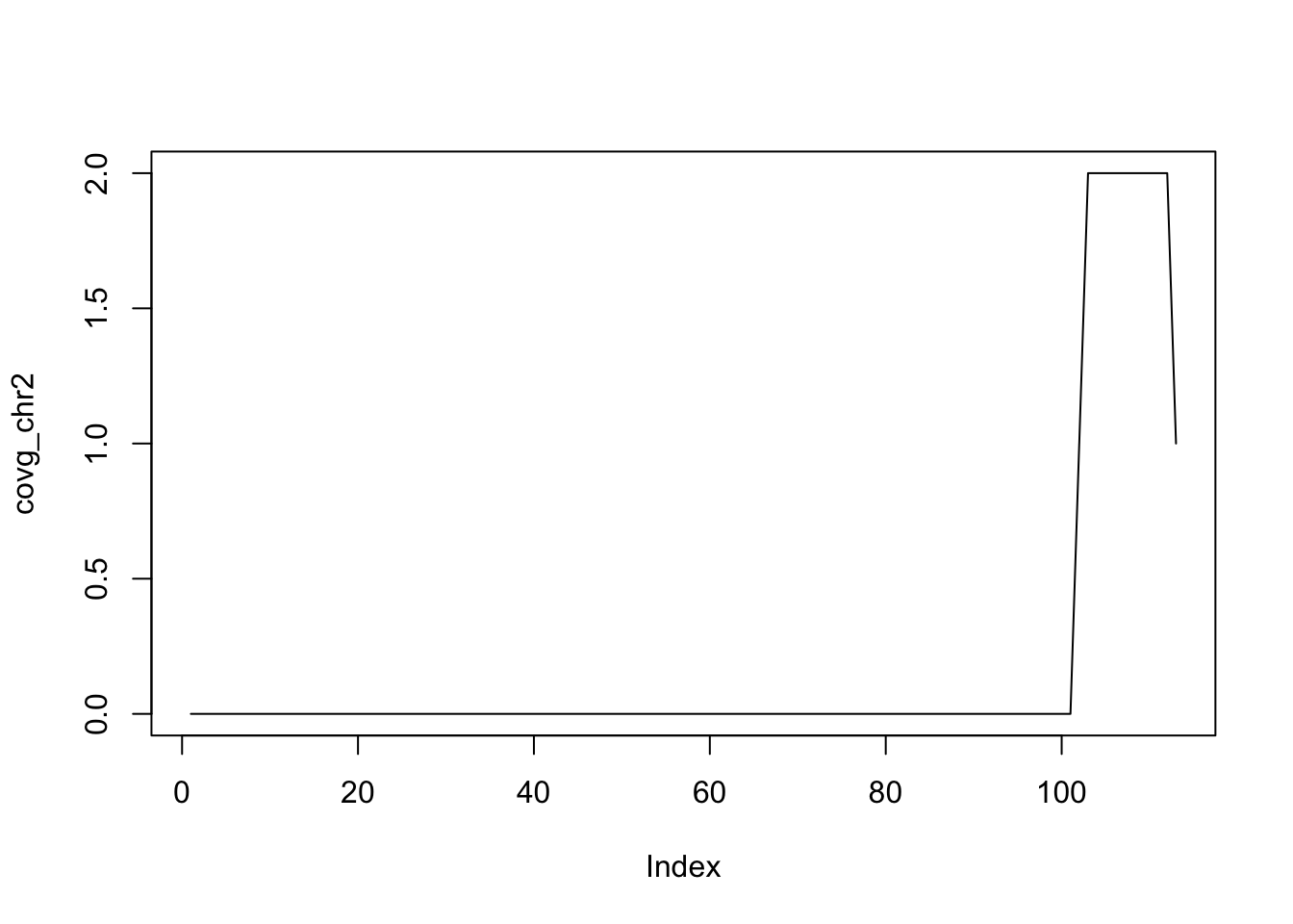
See the GenomicRanges
help page ?"intra-range-methods" for more details.
Set operations for GRanges objects
Between-range methods calculate relationships between different GRanges objects. Of central importance are findOverlaps and related operations; these are discussed below. Additional operations treat GRanges as mathematical sets of coordinates; union(g, g2) is the union of the coordinates in g and g2. Here are examples for calculating the union, the intersect and the asymmetric difference (using setdiff).
g2 <- head(gr, n=2)
union(g, g2)
## GRanges object with 2 ranges and 0 metadata columns:
## seqnames ranges strand
## <Rle> <IRanges> <Rle>
## [1] chr1 101-111 -
## [2] chr2 102-113 +
## -------
## seqinfo: 3 sequences from an unspecified genome; no seqlengthsintersect(g, g2)## GRanges object with 2 ranges and 0 metadata columns:
## seqnames ranges strand
## <Rle> <IRanges> <Rle>
## [1] chr1 101-111 -
## [2] chr2 102-112 +
## -------
## seqinfo: 3 sequences from an unspecified genome; no seqlengthssetdiff(g, g2)## GRanges object with 1 range and 0 metadata columns:
## seqnames ranges strand
## <Rle> <IRanges> <Rle>
## [1] chr2 113 +
## -------
## seqinfo: 3 sequences from an unspecified genome; no seqlengthsThere is extensive additional help available or by looking at the vignettes in at the GenomicRanges pages.
?GRangesThere are also many possible methods that work with
GRanges objects. To see a complete list (long), try:
methods(class="GRanges")GRangesList
Some important genomic features, such as spliced transcripts that are
are comprised of exons, are inherently compound structures. Such a
feature makes much more sense when expressed as a compound object such
as a GRangesList. If we thing of each transcript as a set of exons, each
transcript would be summarized as a GRanges object.
However, if we have multiple transcripts, we want to somehow keep them
separate, with each transcript having its own exons. The
GRangesList is then a list of GRanges objects
that. Continuing with the transcripts thought, a
GRangesList can contain all the transcripts and their
exons; each transcript is an element in the list.
Whenever genomic features consist of multiple ranges that are grouped by a parent feature, they can be represented as a GRangesList object. Consider the simple example of the two transcript GRangesList below created using the GRangesList constructor.
gr1 <- GRanges(
    seqnames = "chr2",
    ranges = IRanges(103, 106),
    strand = "+",
    score = 5L, GC = 0.45)
gr2 <- GRanges(
    seqnames = c("chr1", "chr1"),
    ranges = IRanges(c(107, 113), width = 3),
    strand = c("+", "-"),
    score = 3:4, GC = c(0.3, 0.5))
The gr1 and gr2 are each
GRanges objects. We can combine them into a “named”
GRangesList like so:
grl <- GRangesList("txA" = gr1, "txB" = gr2)
grl
## GRangesList object of length 2:
## $txA
## GRanges object with 1 range and 2 metadata columns:
## seqnames ranges strand | score GC
## <Rle> <IRanges> <Rle> | <integer> <numeric>
## [1] chr2 103-106 + | 5 0.45
## -------
## seqinfo: 2 sequences from an unspecified genome; no seqlengths
##
## $txB
## GRanges object with 2 ranges and 2 metadata columns:
## seqnames ranges strand | score GC
## <Rle> <IRanges> <Rle> | <integer> <numeric>
## [1] chr1 107-109 + | 3 0.3
## [2] chr1 113-115 - | 4 0.5
## -------
## seqinfo: 2 sequences from an unspecified genome; no seqlengthsThe show method for a GRangesList object
displays it as a named list of GRanges objects, where the
names of this list are considered to be the names of the grouping
feature. In the example above, the groups of individual exon ranges are
represented as separate GRanges objects which are further
organized into a list structure where each element name is a transcript
name. Many other combinations of grouped and labeled
GRanges objects are possible of course, but this example is
a common arrangement.
In some cases, GRangesLists behave quite similarly to
GRanges objects.
Basic GRangesList accessors
Just as with GRanges object, the components of the genomic coordinates within a GRangesList object can be extracted using simple accessor methods. Not surprisingly, the GRangesList objects have many of the same accessors as GRanges objects. The difference is that many of these methods return a list since the input is now essentially a list of GRanges objects. Here are a few examples:
seqnames(grl)## RleList of length 2
## $txA
## factor-Rle of length 1 with 1 run
## Lengths: 1
## Values : chr2
## Levels(2): chr2 chr1
##
## $txB
## factor-Rle of length 2 with 1 run
## Lengths: 2
## Values : chr1
## Levels(2): chr2 chr1ranges(grl)## IRangesList object of length 2:
## $txA
## IRanges object with 1 range and 0 metadata columns:
## start end width
## <integer> <integer> <integer>
## [1] 103 106 4
##
## $txB
## IRanges object with 2 ranges and 0 metadata columns:
## start end width
## <integer> <integer> <integer>
## [1] 107 109 3
## [2] 113 115 3strand(grl)## RleList of length 2
## $txA
## factor-Rle of length 1 with 1 run
## Lengths: 1
## Values : +
## Levels(3): + - *
##
## $txB
## factor-Rle of length 2 with 2 runs
## Lengths: 1 1
## Values : + -
## Levels(3): + - *The length and names methods will return the length or names of the list and the seqlengths method will return the set of sequence lengths.
length(grl)## [1] 2names(grl)## [1] "txA" "txB"seqlengths(grl)## chr2 chr1
## NA NARelationships between region sets
One of the more powerful approaches to genomic data integration is to
ask about the relationship between sets of genomic ranges. The key
features of this process are to look at overlaps and distances to the
nearest feature. These functionalities, combined with the operations
like flank and resize, for instance, allow
pretty useful analyses with relatively little code. In general, these
operations are very fast, even on thousands to millions of
regions.
Overlaps
mtch <- findOverlaps(gr, g)
as.matrix(mtch)
## queryHits subjectHits
## [1,] 1 1
## [2,] 2 2
## [3,] 2 3
## [4,] 3 2
## [5,] 3 3
## [6,] 4 2
## [7,] 4 3
## [8,] 5 1If you are interested in only the queryHits or the
subjectHits, there are accessors for those (ie.,
queryHits(match)).
As you might expect, the countOverlaps method counts the
regions in the second GRanges that overlap with those that
overlap with each element of the first.
countOverlaps(gr, g)## a b c d e f g h i j
## 1 2 2 2 1 0 0 0 0 0The subsetByOverlaps method simply subsets the first
GRanges object to include only those that overlap
the second.
subsetByOverlaps(gr, g)## GRanges object with 5 ranges and 3 metadata columns:
## seqnames ranges strand | score GC AT
## <Rle> <IRanges> <Rle> | <integer> <numeric> <numeric>
## a chr1 101-111 - | 1 1.000000 0.000000
## b chr2 102-112 + | 2 0.888889 0.111111
## c chr2 103-113 + | 3 0.777778 0.222222
## d chr2 104-114 * | 4 0.666667 0.333333
## e chr1 105-115 * | 5 0.555556 0.444444
## -------
## seqinfo: 3 sequences from an unspecified genome; no seqlengthsIn some cases, you may be interested in only one hit when doing
overlaps. Note the select parameter. See the help for
findOverlaps
findOverlaps(gr, g, select="first")## [1] 1 2 2 2 1 NA NA NA NA NAfindOverlaps(g, gr, select="first")## [1] 1 2 2The %over% logical operator allows us to do similar
things to findOverlaps and
subsetByOverlaps.
gr %over% g## [1] TRUE TRUE TRUE TRUE TRUE FALSE FALSE FALSE FALSE FALSEgr[gr %over% g]## GRanges object with 5 ranges and 3 metadata columns:
## seqnames ranges strand | score GC AT
## <Rle> <IRanges> <Rle> | <integer> <numeric> <numeric>
## a chr1 101-111 - | 1 1.000000 0.000000
## b chr2 102-112 + | 2 0.888889 0.111111
## c chr2 103-113 + | 3 0.777778 0.222222
## d chr2 104-114 * | 4 0.666667 0.333333
## e chr1 105-115 * | 5 0.555556 0.444444
## -------
## seqinfo: 3 sequences from an unspecified genome; no seqlengthsNearest feature
There are a number of useful methods that find the nearest feature (region) in a second set for each element in the first set.
We can review our two GRanges toy objects:
g## GRanges object with 3 ranges and 3 metadata columns:
## seqnames ranges strand | score GC AT
## <Rle> <IRanges> <Rle> | <integer> <numeric> <numeric>
## a chr1 101-111 - | 1 1.000000 0.000000
## b chr2 102-112 + | 2 0.888889 0.111111
## c chr2 103-113 + | 3 0.777778 0.222222
## -------
## seqinfo: 3 sequences from an unspecified genome; no seqlengthsgr## GRanges object with 10 ranges and 3 metadata columns:
## seqnames ranges strand | score GC AT
## <Rle> <IRanges> <Rle> | <integer> <numeric> <numeric>
## a chr1 101-111 - | 1 1.000000 0.000000
## b chr2 102-112 + | 2 0.888889 0.111111
## c chr2 103-113 + | 3 0.777778 0.222222
## d chr2 104-114 * | 4 0.666667 0.333333
## e chr1 105-115 * | 5 0.555556 0.444444
## f chr1 106-116 + | 6 0.444444 0.555556
## g chr3 107-117 + | 7 0.333333 0.666667
## h chr3 108-118 + | 8 0.222222 0.777778
## i chr3 109-119 - | 9 0.111111 0.888889
## j chr3 110-120 - | 10 0.000000 1.000000
## -------
## seqinfo: 3 sequences from an unspecified genome; no seqlengthsnearest: Performs conventional nearest neighbor finding. Returns an integer vector containing the index of the nearest neighbor range in subject for each range in x. If there is no nearest neighbor NA is returned. For details of the algorithm see the man page in the IRanges package (?nearest).
precede: For each range in x, precede returns the index of the range in subject that is directly preceded by the range in x. Overlapping ranges are excluded. NA is returned when there are no qualifying ranges in subject.
follow: The opposite of precede, follow returns the index of the range in subject that is directly followed by the range in x. Overlapping ranges are excluded. NA is returned when there are no qualifying ranges in subject.
Orientation and strand for precede and follow: Orientation is 5’ to 3’, consistent with the direction of translation. Because positional numbering along a chromosome is from left to right and transcription takes place from 5’ to 3’, precede and follow can appear to have ‘opposite’ behavior on the + and - strand. Using positions 5 and 6 as an example, 5 precedes 6 on the + strand but follows 6 on the - strand.
The table below outlines the orientation when ranges on different strands are compared. In general, a feature on * is considered to belong to both strands. The single exception is when both x and subject are * in which case both are treated as +.
       x  |  subject  |  orientation
     -----+-----------+----------------
a)     +  |  +        |  --->
b)     +  |  -        |  NA
c)     +  |  *        |  --->
d)     -  |  +        |  NA
e)     -  |  -        |  <---
f)     -  |  *        |  <---
g)     *  |  +        |  --->
h)     *  |  -        |  <---
i)     *  |  *        |  --->  (the only situation where * arbitrarily means +)
res = nearest(g, gr)
res## [1] 5 4 4While nearest and friends give the index of the nearest
feature, the distance to the nearest is sometimes also useful to have.
The distanceToNearest method calculates the nearest feature
as well as reporting the distance.
res = distanceToNearest(g, gr)
res
## Hits object with 3 hits and 1 metadata column:
## queryHits subjectHits | distance
## <integer> <integer> | <integer>
## [1] 1 5 | 0
## [2] 2 4 | 0
## [3] 3 4 | 0
## -------
## queryLength: 3 / subjectLength: 10Session Info
sessionInfo()## R version 4.2.0 (2022-04-22)
## Platform: x86_64-apple-darwin17.0 (64-bit)
## Running under: macOS Big Sur/Monterey 10.16
##
## Matrix products: default
## BLAS: /Library/Frameworks/R.framework/Versions/4.2/Resources/lib/libRblas.0.dylib
## LAPACK: /Library/Frameworks/R.framework/Versions/4.2/Resources/lib/libRlapack.dylib
##
## locale:
## [1] en_US.UTF-8/en_US.UTF-8/en_US.UTF-8/C/en_US.UTF-8/en_US.UTF-8
##
## attached base packages:
## [1] stats4 stats graphics grDevices utils datasets methods
## [8] base
##
## other attached packages:
## [1] GenomicRanges_1.48.0 GenomeInfoDb_1.32.0 IRanges_2.30.0
## [4] S4Vectors_0.34.0 BiocGenerics_0.42.0 BiocStyle_2.24.0
## [7] knitr_1.39
##
## loaded via a namespace (and not attached):
## [1] rstudioapi_0.13 XVector_0.36.0 magrittr_2.0.3
## [4] zlibbioc_1.42.0 R6_2.5.1 rlang_1.0.2
## [7] fastmap_1.1.0 highr_0.9 stringr_1.4.0
## [10] tools_4.2.0 xfun_0.30 cli_3.3.0
## [13] jquerylib_0.1.4 htmltools_0.5.2 yaml_2.3.5
## [16] digest_0.6.29 GenomeInfoDbData_1.2.8 BiocManager_1.30.17
## [19] bitops_1.0-7 sass_0.4.1 RCurl_1.98-1.6
## [22] evaluate_0.15 rmarkdown_2.14 stringi_1.7.6
## [25] compiler_4.2.0 bslib_0.3.1 jsonlite_1.8.0